미분다양체
Vector Fields
Vector fields
This post was machine-translated from the Korean original by Marvin (via Kimi). It may contain errors or awkward phrasing — the Korean original is the source of truth.
Vector Fields
We defined vector bundles in the previous post partly for later use, but we also needed them immediately to define vector fields.
Definition 1 For any vector bundle \(\pi:E\rightarrow M\), a map \(\sigma:M\rightarrow E\) satisfying \(\pi\circ\sigma=\id_M\) is called a section of the vector bundle \(E\rightarrow M\).
This definition merely says that \(\sigma\) is a function taking each point \(p\) to an element of \(E_p\). Meanwhile, since \(E\) is itself a manifold, any section \(\sigma:M\rightarrow E\) is a map between two manifolds, and thus the smoothness of \(\sigma\) is well-defined. We write \(\Gamma(E)\) for the set of smooth sections of the vector bundle \(E\rightarrow M\).
In particular, a section \(X\) of the tangent bundle \(\pi:TM\rightarrow M\) is called a vector field, and the value of \(X\) at a point \(p\) is often written \(X_p\). Since \(X_p\in T_pM\), for a function \(f\) defined near \(p\), the real number \(X_p(f)\) is well-defined. In particular, if \(f\) is defined on an open set \(U\), we denote by \(X(f)\) the function \(U\rightarrow\mathbb{R}\) sending \(p\in U\) to the real number \(X_p(f)\).
Proposition 2 Let \(X\) be a vector field on a manifold \(M\). Then the following are equivalent.
- \(X\) is \(C^\infty\).
-
For any coordinate system \((U,\varphi)\), \(\varphi=(x^i)_{i=1}^m\), the functions \(a^i:U\rightarrow\mathbb{R}\) defined by the formula
\[(X\vert_U)_p=\sum_{i=1}^m a^i(p)\frac{\partial}{\partial x^i}\bigg\vert_p\]are all \(C^\infty\) on \(U\).
- For any open set \(V\subseteq M\) and any \(C^\infty\) function \(f:V\rightarrow\mathbb{R}\), the function \(X(f)\) is also \(C^\infty\).
Proof
First, if \(X\) is \(C^\infty\), then clearly \(X\vert_U\) is \(C^\infty\). Meanwhile, as functions on \(TM\), the \(dx^i\) are component functions of the coordinate system \(\tilde{\varphi}:\pi^{-1}(U)\rightarrow\mathbb{R}^{2m}\), so they are likewise \(C^\infty\), and therefore their composition
\[a^i(p)=dx^i\left(\sum a^i(p)\frac{\partial}{\partial x^i}\bigg\vert_p\right)=dx^i\vert_p\circ(X\vert_U)_p\]is also obviously \(C^\infty\).
Assume condition 2 holds. To show that \(X(f)\) is \(C^\infty\) at any \(p\in V\), it suffices to show that \(X(f)\) is \(C^\infty\) at \(p\) for some coordinate system \((U,\varphi)\) containing \(p\). By condition 2,
\[(X\vert_U)_pf=\sum_{i=1}^m a^i(p)\frac{\partial f}{\partial x^i}(p)\]and the right-hand side is a \(C^\infty\) function on \(U\), so \(X(f)\) is \(C^\infty\).
Finally, assume condition 3 and show 1. To show that \(X:M\rightarrow TM\) is \(C^\infty\), it suffices to show that for any coordinate system \((U,\varphi)\), the map \(X\circ\varphi^{-1}\) is a \(C^\infty\) map from \(\varphi(U)\) to \(TM\); considering the coordinate system on \(TM\), this amounts to showing that the functions
\[x^i\circ\pi\circ (X\vert_U),\quad dx^i\circ(X\vert_U)\]are \(C^\infty\). But direct computation gives
\[x^i\circ\pi\circ (X\vert_U)=x^i\circ\id_U=x^i,\qquad dx^i\circ(X\vert_U)=X(x^i)\]so they are all \(C^\infty\).
We write \(\mathfrak{X}(M)\) for the set of \(C^\infty\) vector fields on \(M\), and henceforth assume all vector fields are \(C^\infty\). Meanwhile, by a partition of unity, any vector field defined only on some open set \(U\) of \(M\) can be extended to all of \(M\). (§Tangent Space)
Local Frame
Addition of two elements \(X,Y\) in \(\mathfrak{X}(M)\) is well-defined by
\[(X+Y)_p=X_p+Y_p\]and for any real number \(\alpha\in\mathbb{R}\), defining
\[(\alpha X)_p=\alpha\cdot X_p\]we see that \(\alpha X\) is also an element of \(\mathfrak{X}(M)\). Thus \(\mathfrak{X}(M)\) is an \(\mathbb{R}\)-vector space. However, as an \(\mathbb{R}\)-vector space, \(\mathfrak{X}(M)\) is too large.
Example 3 Let \(M=\mathbb{R}\). Here we regard \(M\) as equipped with the manifold structure given by the single chart \((\mathbb{R},\id)\). Then the tangent space \(T_pM\) at each point \(p\) is the one-dimensional vector space spanned by \(d/dx\vert_p\), and thus the correspondence
\[X:M\rightarrow TM;\qquad p\mapsto \frac{d}{dx}\bigg\vert_p\]is an element of \(\mathfrak{X}(M)\). However, for any \(C^\infty\) function \(f:\mathbb{R}\rightarrow\mathbb{R}\),
\[fX:M\rightarrow TM;\qquad p\mapsto f(p)\frac{d}{dx}\bigg\vert_p\]also belongs to \(\mathfrak{X}(M)\) (Proposition 2), and this element cannot be expressed as a constant multiple of \(X\) unless \(f\) is constant. Moreover, since \(C^\infty(M)\) is an infinite-dimensional vector space over \(\mathbb{R}\), the space \(\mathfrak{X}(M)\) is also infinite-dimensional.
In such a situation, it is relatively more convenient to regard \(\mathfrak{X}(M)\) as a \(C^\infty(M)\)-module.
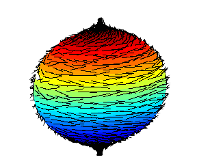
In the example above, \(\mathfrak{X}(M)\) was generated by the single vector field \(d/dx\), but in general, since \(C^\infty(M)\) is not a field, there can very well exist \(C^\infty(M)\)-modules without a basis. For instance, the well-known hairy ball theorem shows that any continuous vector field on the unit sphere \(S^2\) in 3-dimensional space must vanish at some point.
Suppose two vector fields \(X_1,X_2\) on the 2-manifold \(M=S^2\) generate \(\mathfrak{X}(M)\) as a \(C^\infty(M)\)-module. Then by the hairy ball theorem, there exists a point \(p\in S^2\) with \(X_1(p)=0\). Then \(T_pM\) would have to be generated by \(\{0,X_2(p)\}\), which contradicts the fact that \(T_pM\) is 2-dimensional. Therefore, \(\mathfrak{X}(M)\) cannot be generated by two vector fields \(\{X_1,X_2\}\).
On the other hand, for a sufficiently small open set \(U\), the set \(\mathfrak{X}(U)\) of vector fields on \(U\) can be regarded as a \(C^\infty(U)\)-module generated by \(m\) vector fields. For the tangent bundle \(\pi: TM\rightarrow M\), if we take \(U\) sufficiently small, we can find a diffeomorphism \(h:U\times\mathbb{R}^m\rightarrow\pi^{-1}(U)\); defining vector fields \(X_1,\ldots, X_m\) by
\[X_1(p)=h(p, e_1),\quad X_2(p)=h(p,e_2),\quad\ldots,\quad X_m(p)=h(p,e_m)\tag{1}\]these generate \(\mathfrak{X}(U)\).
Definition 4 Let \(M\) be a manifold, and let \(\dim M=m\).
- We say that \(X_1,\ldots, X_k\) are linearly independent on a subset \(A\) of \(M\) if for each \(p\in A\), the vectors \(X_1(p),\ldots, X_k(p)\) in \(T_pM\) are linearly independent.
- We say that \(X_1,\ldots, X_k\) span the tangent bundle \(TM\) on a subset \(A\) of \(M\) if for each \(p\in A\), the vectors \(X_1(p),\ldots, X_k(p)\) in \(T_pM\) span \(T_pM\).
- If linearly independent vector fields \(X_1,\ldots, X_k\) on an open set \(U\subseteq M\) span the tangent bundle, we call them a local frame of \(M\).
- If in the above definition we can take \(U=M\), we call these vector fields a global frame of \(M\).
Therefore, from the above discussion we see that a parallelizable manifold admits a global frame. Conversely, if a manifold \(M\) has a global frame \(X_1,\ldots, X_m\), we can verify that \(M\) is parallelizable by defining a map \(TM\rightarrow M\times\mathbb{R}^m\) by
\[(p,a_1X_1(p)+\cdots+a_mX_m(p))\mapsto (p,a_1e_1+\cdots+a_me_m)\]Integral Flow
Definition 5 A \(C^\infty\) curve \(\sigma\) on a manifold \(M\) is called an integral flow of \(X\in\mathfrak{X}(M)\) if \(\sigma'(t)=X(\sigma(t))\) holds for all \(t\).
The following theorem follows easily from the theory of ordinary differential equations, but we omit its proof since it lies beyond our scope. Moreover, from item 4 onward, the theorem requires a few additional definitions.
Theorem 6 Let \(M\) be a manifold and let \(X\in\mathfrak{X}(M)\). For each \(p\in M\), there exist suitable constants \(a(p), b(p)\) (possibly \(\pm\infty\)) and a \(C^\infty\) curve \(\phi_p: \bigl(a(p),b(p)\bigr)\rightarrow M\) satisfying the following conditions.
- \(0\in \bigl(a(p),b(p)\bigr)\), \(\phi_p(0)=p\).
- \(\phi_p\) is an integral flow of \(X\).
- If \(\mu:(c,d)\rightarrow M\) is a \(C^\infty\) function satisfying the above two conditions, then \((c,d)\subseteq \bigl(a(p),b(p)\bigr)\), and \(\mu\) coincides with the restriction of \(\phi_p\) to \((c,d)\).
- For each \(p\in M\), there exist a suitable open neighborhood \(V\) and a positive number \(\epsilon\) such that \((t,p)\mapsto \phi^{t}(p):=\phi_p(t)\) is well-defined, and this function is a \(C^\infty\) map from \((-\epsilon,\epsilon)\times V\) to \(M\).
- For any \(t\), the set \(\mathcal{D}_t=\left\{p\in M\mid t\in\bigl(a(p),b(p)\bigr)\right\}\) is open.
- \(\bigcup_{t>0}\mathcal{D}_t=M\).
- \(\phi^{t}:\mathcal{D}_t\rightarrow\mathcal{D}_{-t}\) is a diffeomorphism, and its inverse is \(\phi^{-t}\).
- The domain of \(\phi^s\circ \phi^t\) is contained in \(\mathcal{D}_{s+t}\), and in particular, if \(s\) and \(t\) have the same sign, the domain of this function coincides exactly with \(\mathcal{D}_{s+t}\). Moreover, on this domain, \(\phi^s\circ \phi^t=\phi^{t+s}\).
Even though the proof is omitted, we must fully understand what this theorem asserts.
First, items 1 through 3 show that for each \(p\in M\) there corresponds a unique maximal integral flow, which is uniquely determined up to reparametrization of time \(t\).
To understand the remainder of the theorem, we need some additional explanation of the notation. First, the function \(\phi^{t}(p)\) in condition 4 is defined, as in the definition, by
\[\phi^{t}(p)=\phi_p(t)\]and the initial condition fixes \(\phi_p(0)=p\) at time \(0\). We denote the domain of \(\phi^{t}\) by
\[\mathcal{D}_t=\left\{p\in M\mid t\in\bigl(a(p),b(p)\bigr)\right\}\]Thus we may think of \(\phi^{t}\) as the function giving the position, after \(t\) seconds, of the point that started at \(p\) at time \(0\) and moved along the integral flow; accordingly, \(\mathcal{D}_t\) is the set of points for which it is possible to move along the integral flow for \(t\) seconds.
Now, setting aside the technical results 4 and 5, the next statement is 6, which is in fact merely a restatement of the existence of integral flows in a different form. Statement 7 shows that distinct integral flows do not intersect.
Statement 8 also has a somewhat technical aspect: if \(s\) and \(t\) had opposite signs, say \(s=-2\) and \(t=1\), then the domain of \(\phi^s\circ\phi^t\) would not simply be \(\mathcal{D}_{-1}\), but rather the subset of \(\mathcal{D}_{-1}\) consisting of those points for which it is possible to proceed along \(\phi_p\) for 1 second.
Definition 7 We say that \(X\in\mathfrak{X}(M)\) is complete if \(\mathcal{D}_t=M\) for all \(t\). In this case, the maps \(\phi^t\) form a group under composition \(\circ\), called the one-parameter group of \(X\).
If \(X\) is not complete, there is a slight problem with the domains of the \(\phi^t\) as above, making it difficult to regard them as a group. A more subtle case is when the original vector field \(X\) varies with time, but this is not yet our concern, so we pass over it.
References
[War] Frank W. Warner. Foundations of Differentiable Manifolds and Lie Groups, Graduate texts in mathematics, Springer, 2013
[Lee] John M. Lee. Introduction to Smooth Manifolds, Graduate texts in mathematics, Springer, 2012
댓글남기기