Homology

This post was machine-translated from the Korean original by Marvin (via Kimi). It may contain errors or awkward phrasing — the Korean original is the source of truth.

Simplices

First, the simplex we introduce is helpful for intuitive understanding when developing homology theory.

Definition 1 For any natural number \(k\), suppose \(k+1\) points \(v_0,\ldots, v_k\in\mathbb{R}^d\) arranged in general position are given. Then the \(k\)-simplex is the smallest convex set containing the set \(\{v_0,\ldots, v_k\}\).

Here, saying that the \(k+1\) vertices are arranged in general position means that these points are not contained in any hyperplane of dimension less than \(k\). Equivalently, this can also be understood as the \(k\) vectors

\[v_1-v_0,\ldots, v_k-v_0\]

being linearly independent. For example, a \(0\)-simplex is a point, a \(1\)-simplex is a line segment connecting two vertices, a \(2\)-simplex is a triangle connecting three points, and a \(3\)-simplex is a tetrahedron.

As in the figure above, the \(n\)-simplex formed by \(n+1\) vertices in \(\mathbb{R}^{n+1}\)

\[(1,0,\ldots, 0),\qquad\cdots,\qquad (0,0,\ldots,1)\]

is called the standard simplex. Naturally, these simplices themselves are not our objects of interest; we are interested in using them to compute invariants of manifolds. For this purpose, we need to define a \(\Delta\)-complex structure on a manifold, but let us first look at a simple and intuitive example.

Example 2 An example we often think of is the (2-dimensional) torus \(T^2\). By a simple definition this is the product manifold \(S^1\times S^1\), but to intuitively see that this product manifold is a torus, we can think of the following figure.

In this figure, imagine gluing the edges of each color together in the direction of the arrows “without twisting.” For instance, if we first glue the horizontal edges to form a cylinder, and then glue the remaining edges along the top and bottom of the cylinder together, we obtain the following.

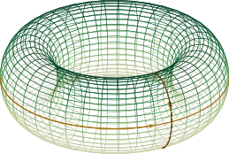
This is the quotient space obtained by imposing the following equivalence relation on the square, if it were the square on the coordinate plane passing through the four points \((0,0),(0,1),(1,0),(1,1)\):

\[(x,0)\sim (x,1),\qquad (0,y)\sim(1,y)\]

and if we think of \(S^1\) as obtained by giving the quotient topology on the interval \([0,1]\) on the real line by identifying \(0\) and \(1\), we see that this is the same as the above definition \(T^2=S^1\times S^1\). On the other hand, if on the same figure we reverse the direction of one edge and glue only the horizontal edges, we obtain the following quotient space

and the space obtained this time is not a cylinder but the Möbius strip

.

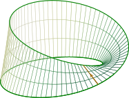
In the above example, if we divide the squares drawn on the plane into two triangles along a diagonal, these squares can be thought of as two \(2\)-simplices glued together, and if we carry this over to the quotient space in the same way as above, we can understand the spaces of Example 2 as being made by gluing simplices together. As can be seen from this example, when gluing \(2\)-simplices the direction of the edge (more generally, when gluing \(n\)-simplices the direction of the \((n-1)\)-simplex) is important, and this is determined by giving a total order among the vertices. For example, if we say that the \(k\)-simplex formed by vertices \(v_0,\ldots, v_k\) listed in order of indices is the positive direction, then \(v_1,v_0,v_2,\ldots,v_k\) obtained by taking an odd permutation is the negative direction, and so on. We write a simplex with orientation given according to the index order as \([v_0,\ldots, v_k]\). Under this notation, if we forget the vertex \(v_i\) of the \(k\)-simplex and give orientation to the resulting face by restricting the total order of the original vertices, this is the same as the orientation of the following \((k-1)\)-simplex

\[[v_0,\ldots,\hat{v}_i,\ldots, v_k]=[v_0,\ldots, v_{i-1},v_{i+1},\ldots, v_k]\]

.

Definition 3 For a topological space \(X\), a \(\Delta\)-complex structure on it is a collection of functions \(\sigma_\alpha:\Delta^{n(\alpha)}\rightarrow X\) defined as follows.

1. The restriction of \(\sigma_\alpha\) to \(\interior(\Delta^{n(\alpha)})\) is injective, and for any point \(x\) in \(X\) there exists exactly one \(\alpha\) such that \(x\in \sigma_\alpha(\interior(\Delta^{n(\alpha)}))\).
2. The restriction of \(\sigma_\alpha\) to a face of \(\Delta^{n(\alpha)}\), \(\sigma_\alpha\vert_{\Delta^{n(\alpha)-1}}:\Delta^{n(\alpha)-1}\rightarrow X\), also belongs to this collection of functions.
3. \(A\subseteq X\) is an open set in \(X\) if and only if \(\sigma_\alpha^{-1}(A)\) is an open set in \(\Delta^{n(\alpha)}\) for each \(\alpha\).

For example, the standard simplex \(\Delta^2\) trivially has a \(\Delta\)-complex structure, and the functions explicitly giving this structure are

\[\id_{\Delta^2}:\Delta^2\rightarrow\Delta^2\]

together with three functions \(\sigma^1_1,\sigma^1_2,\sigma^1_3\) sending the \(1\)-simplex \(\Delta^1\) to each edge, and three functions \(\sigma_1^0,\sigma_2^0,\sigma_3^0\) sending the \(0\)-simplex \(\Delta^0\) to each vertex.

Example 4 For example, the 2-dimensional torus \(T^2\) can be represented as in the following figure

and this figure simultaneously gives a \(\Delta\)-complex structure on \(T^2\).

Simplicial Homology

Now we define invariants of topological spaces using the \(\Delta\)-complex structure defined above. More specifically, this will be defined through the group formed by formal sums of simplices. However, there is a subtle issue to point out at this stage: for this to be an invariant of the topological space \(X\), it must not depend on the choice of \(\Delta\)-complex structure.

For example, if we subdivide the square of Example 2 more finely to create more 2-simplices as in the figure above, the new gray \(1\)-simplices that arise from this must somehow cancel each other out. That is, when choosing a \(\Delta\)-complex we must glue them together with appropriate matching directions, but when computing invariants we must add them with opposite signs. Keeping this in mind, the following calculation will make somewhat more sense.

Consider a topological space \(X\) with a given \(\Delta\)-complex structure, and consider the free abelian group \(C^\Delta_k(X)\) generated by the \(k\)-simplices. That is,

\[C^\Delta_k(X)=\{\sigma_\alpha:\Delta^{n(\alpha)}\rightarrow X\text{ $k$-simplex}\mid n(\alpha)=k\}\cdot\mathbb{Z}\]

.¹ Following the convention when dealing with abelian groups, we think of the operation on \(C^\Delta_k(X)\) as given by addition. As we saw earlier, the boundary of the \(k\)-simplex \([v_0,\ldots, v_k]\) consists of the following \((k-1)\)-simplices:

\[[v_1,v_2,\ldots, v_k],\quad[v_0,v_2,\ldots, v_k],\quad\cdots,[v_0,v_1,\ldots\hat{v}_i,\ldots,v_k],\quad\cdots,\quad[v_0,v_1,\ldots, v_{k-1}]\]

If we think of the boundary of \([v_0,\ldots, v_k]\) as the sum of these, we obtain a function from \(C^\Delta_k(X)\) to \(C^\Delta_{k-1}(X)\). If we define the boundary map \(\partial_k\) not as a simple sum of these simplices but by the following formula

\[\partial_k(\sigma_\alpha\vert_{[v_0,\ldots,v_k]})=\sum_{i=0}^k(-1)^i\sigma_\alpha\vert_{[v_0,\ldots, \hat{v}_i,\ldots,v_k]}\tag{1}\]

then it is well known that \((C^\Delta_k(X),\partial_k)\) forms a chain complex. The signs on the right-hand side of this formula are, as pointed out above, set up so that adjacent simplices inside \(X\) cancel each other out.

Proposition 5 \((C^\Delta_k(X),\partial_k)\) is a chain complex. ([Category Theory] §Abelian Categories, ⁋Definition 4)

Proof

For any \(\sigma_\alpha\in C^\Delta_k(X)\), since

\[\partial_k(\sigma_\alpha\vert_{[v_0,\ldots,v_k]})=\sum_{i=0}^k(-1)^i\sigma_\alpha\vert_{[v_0,\ldots, \hat{v}_i,\ldots,v_k]}\]

we have

\[\partial_{k-1}\partial_k(\sigma_\alpha\vert_{[v_0,\ldots,v_k]})=\sum_{j < i}(-1)^{i+j}\sigma_\alpha\vert_{[v_0,\ldots, \hat{v}_j,\ldots\hat{v}_i,\ldots,v_k]}+\sum_{j > i}(-1)^{i+j-1}\sigma_\alpha\vert_{[v_0,\ldots, \hat{v}_i,\ldots\hat{v}_j,\ldots,v_k]}\]

and thus the first sum and the second sum cancel each other out and vanish.

The \(n\)th homology of the chain complex \((C^\Delta_k(X),\partial_k)\) obtained in this way is called the \(n\)-th simplicial homology, and we write it as \(H_n^\Delta(X)\). ([Homological Algebra] §Homology, ⁋Definition 2)

Example 6 Represent the 2-dimensional torus \(T^2\) as in Example 4 above, and let the \(2\)-simplices in the order listed on the right be \(L\), \(U\), the \(1\)-simplices be \(a,b,c\), and the \(0\)-simplex be \(p\). Since directions are already given to the two \(1\)-simplices \(b,c\), for these to be simplices \(a\) must have the direction from lower left to upper right. Now, if we think of the vertices \(v_0,v_1,v_2\) of \(U\) as given as in

then we can set

\[a=[v_0,v_2],\quad b=[v_1,v_2],\quad c=[v_0,v_1]\]

Similarly, if we think of the vertices \(v_0,v_1,v_2\) of \(L\) as given as in the following figure

then for \(L\) we can think of

\[a=[v_0,v_2],\quad b=[v_0,v_1],\quad c=[v_1,v_2]\]

Now, considering the boundary map \(\partial_2:C^\Delta_2(T^2)\rightarrow C^\Delta_1(T^2)\), we have

\[\begin{aligned}\partial_2(U)&=[v_1,v_2]-[v_0,v_2]+[v_0,v_1]=b-a+c,\\ \partial_2(L)&=[v_1,v_2]-[v_0,v_2]+[v_0,v_1]=c-a+b\end{aligned}\]

Also, considering \(\partial_1:C^\Delta_1(T^2)\rightarrow C^\Delta_0(T^2)\), since all these vertices correspond to the same point \(p\) in \(T^2\), we have

\[\partial_1(a)=\partial_1(b)=\partial_1(c)=p-p=0\]

and thus in the following complex

\[\cdots\overset{\partial_3}{\longrightarrow}C^\Delta_2(T^2)=\langle L,U\rangle\overset{\partial_2}{\longrightarrow}C^\Delta_1(T^2)=\langle a,b,c\rangle\overset{\partial_1}{\longrightarrow}C^\Delta_0(T^2)=\langle p\rangle\overset{\partial_0}{\longrightarrow}0\]

we have

\[\ker\partial_2=\langle L-U\rangle,\qquad\ker\partial_1=C^\Delta_1(T^2),\qquad\ker\partial_0=C^\Delta_0(T^2)\]

and

\[\im\partial_3=0,\qquad\im\partial_2=\langle a-b-c\rangle,\qquad \im\partial_1=0\]

so

\[H_2^\Delta(T^2)=\ker\partial_2/\im\partial_3\cong\mathbb{Z},\quad H_1^\Delta(T^2)=\ker\partial_1/\im\partial_2\cong \mathbb{Z}\oplus\mathbb{Z},\quad H_0^\Delta(T^2)=\ker\partial_0/\im\partial_1\cong\mathbb{Z}\]

and the remaining homology is all \(0\).

Meanwhile, in [Homological Algebra] §Homology, ⁋Definition 2, we called the elements of \(Z_n(C)=\ker\partial_n\) \(n\)-cycles and the elements of \(B_n(C)=\im\partial_{n+1}\) \(n\)-boundaries, and now those names are intuitively clear. That is, in this case the boundary maps actually compute the boundary faces of simplices, \(n\)-cycles mean those whose values cancel out when computing boundary faces in this way, for example in Example 6 they mean things like the closed curves formed by \(a,b\) (and \(c\)) in the original space \(T^2\), and \(n\)-boundaries literally mean the \(n\)-simplices that appear as the boundary of some \((n+1)\)-simplex.

Singular Homology

The simplicial homology defined above has an intuitively clear meaning, but its limitation is evident in that to compute the homology of an arbitrary topological space \(X\), we must give a \(\Delta\)-complex structure on it. It is well known that even if \(X\) is a topological manifold, if its dimension is \(4\) or higher, it may be impossible to give a \(\Delta\)-complex structure on \(X\).

Therefore we relax this condition and define a new homology.

Definition 7 A singular \(k\)-simplex defined on \(X\) means a continuous function \(\sigma:\Delta^k\rightarrow X\).

Unlike the \(\Delta\)-complex structure defined earlier, singular \(k\)-simplices do not need to maintain the shape of a \(k\)-simplex at all inside \(X\). For example, a constant map sending all points of \(\Delta^k\) to a single point is also a singular \(k\)-simplex.

Now let \(C_k(X)\) be the free abelian group generated by all singular \(k\)-simplices, and define \(\partial_k:C_k(X)\rightarrow C_{k-1}(X)\) in the same way as in formula (1) above. Then we can verify in exactly the same way as in Proposition 5 that \((C_k(X), \partial_k)\) becomes a chain complex, and we call the homology in this case singular homology and write it as \(H_n(X)\).

Example 8 Computing singular homology directly from the definition is not a good idea, but let us do some (non-rigorous) calculation for our intuition.

By definition, a singular \(0\)-simplex on an arbitrary topological space \(X\) is a continuous function from \(\Delta^0\) to \(X\). But since \(\Delta^0\) is just a single point, \(C_0(X)\) is the free abelian group generated by the points of \(X\). Similarly, if we identify \(\Delta^1\) with the interval \(I=[0,1]\), then \(C_1(X)\) is just the free abelian group generated by paths in \(X\), and in this case we also allow constant paths \([0,1]\rightarrow X\), and for this reason we call this a singular \(1\)-simplex. Likewise, after continuous deformation, \(C_2(X)\) will be the free abelian group generated by disks contained in \(X\).

Then the boundary of a path \(\sigma:[0,1]\rightarrow X\) is given by \(\partial_1\sigma=\sigma(1)-\sigma(0)\) according to formula (1), and from this we know that

\[Z_1(X)=\ker\partial_1\supseteq\left\{\sigma:[0,1]\rightarrow X\mid \sigma(1)=\sigma(0)\right\}\]

That is, intuitively we can think of \(Z_1(X)\) as the subgroup generated by closed curves in \(X\). Similarly, if we give geometric meaning to \(B_1(X)=\im\partial_2\), this means closed curves in \(X\) that arise as the boundary of some disk, and therefore the first homology

\[H_1(X)=\frac{Z_1(X)}{B_1(X)}\]

examines how many closed curves in \(X\) exist that do not arise as the boundary of a disk. For example, the first homology of the subset of \(\mathbb{R}^2\)

\[D^2=\left\{(x,y)\in \mathbb{R}^2\mid x^2+y^2\leq 1\right\}\]

is \(0\). This is because however a closed curve in \(D^2\) is given, there trivially exists a way to fill its interior.

On the other hand, the first homology of the space \(D^2\setminus\left\{(0,0)\right\}\) is not \(0\). For example, considering the following closed curve

there is no way to continuously fill its interior to make it a disk. However, similarly considering the following punctured space

\[D^3\setminus \left\{(0,0,0)\right\}=\left\{(x,y,z)\in \mathbb{R}^3\mid 0< x^2+y^2+z^2\leq 1\right\}\]

the first homology of this space is \(0\), because even if we are given a closed curve “containing the hole”

\[S^1=\left\{(x,y,0)\in \mathbb{R}^3\mid x^2+y^2=1\right\}\]

as in

we can view it as the boundary of a disk. Instead, the second homology of this space will not be \(0\).

There is a slight gap in this calculation. For example, a constant map sending all points of \(\Delta^1\) to a fixed \(x\in X\) is a singular \(1\)-simplex by definition, but when we claim that any closed curve in \(D^2\) can be filled, we did not consider (constant) paths of this form. However, what we need to show is ultimately that applying \(\partial\) to an appropriate singular \(2\)-simplex \(\Delta^2 \rightarrow X\) yields this singular \(1\)-simplex, so if we simply consider a \(2\)-simplex sending all points of \(\Delta^2\) to a fixed \(x\in X\) and then think of its boundary, this is exactly the simplex \(\Delta^1 \rightarrow X\) that we want. Generalizing this, for any odd \(n\), a singular \(n\)-simplex sending all points of \(\Delta^n\) to a fixed \(x\in X\) is the boundary of a singular \((n+1)\)-simplex sending all points of \(\Delta^{n+1}\) to a fixed \(x\in X\). In other words, for odd \(n\), a constant map becomes the identity in \(H_n(X)\).

Gaps of this kind can be resolved with a little care as above. In fact, it can be shown that for any space \(X\) on which a \(\Delta\)-complex structure can be given, the singular homology \(H_n(X)\) and the simplicial homology \(H_n^\Delta(X)\) always agree, and roughly speaking, this is because singular maps \(\Delta^k \rightarrow X\) such as constant maps become boundaries of similarly singular \(\Delta^{k+1}\rightarrow X\), so that when comparing the two quotients

\[H_n^\Delta(X)=\frac{\ker\partial_n^\Delta}{\im\partial_{n+1}^\Delta},\qquad H_n(X)=\frac{\ker\partial_n}{\im\partial_{n+1}}\]

allowing singular \(\Delta^k \rightarrow X\) makes \(\ker \partial_n\) larger than \(\ker\partial_n^\Delta\) by exactly as much as \(\im\partial_{n+1}\) also becomes larger, so that the two quotients end up equal.

A somewhat more fundamental problem is that this calculation relies entirely on our geometric intuition, and to compute the homology of more complicated spaces we need to study more general properties of homology.

Properties of Homology

Proposition 9 When a topological space \(X\) is expressed as the disjoint union \(X=\coprod X_i\) of its path-components, the following isomorphism holds:

\[H_n(X)\cong \bigoplus_{i\in I} H_n(X_i)\]

Proof

First, since the continuous image of a path-connected space \(\Delta^k\) is path-connected, the images of singular simplices lie entirely within the \(X_i\). From this we know that \(C_n(X)\cong \bigoplus_{i\in I} C_n(X_i)\). For the same reason the \(\partial\)’s also preserve this decomposition, and since direct sum preserves the kernel and image of such maps, we obtain the desired result.

Therefore computing the homology of an arbitrary topological space reduces to computing the homology of an arbitrary path-connected space. However, this is still not an easy problem. We cannot compute in the general case, but the case \(n=0\) has geometric meaning.

Proposition 10 For a non-empty path-connected space \(X\), \(H_0(X)\cong \mathbb{Z}\).

Proof

First, since \(\partial_0=0\), we have

\[H_0(X)=\ker\partial_0/\im\partial_1=C_0/\im\partial_1\]

To construct an isomorphism \(H_0(X)\rightarrow\mathbb{Z}\), define a homomorphism \(\varepsilon:C_0(X)\rightarrow\mathbb{Z}\) by the following formula:

\[\varepsilon\left(\sum n_i\sigma_i\right)=\sum_i n_i\]

Then since \(X\) is nonempty, \(\varepsilon\) is surjective. Therefore by the first isomorphism theorem it suffices to show that \(\ker\varepsilon=\im\partial_1\). That \(\ker\varepsilon\) contains \(\im\partial_1\) is trivial from the definition of \(\partial_1\), so it suffices to show the reverse inclusion. Assume \(\varepsilon\left(\sum n_i\sigma_i\right)=0\), and for each \(i\) let \(x_i\) be the image of the \(0\)-simplex \(\sigma_i\). Then by the assumption that \(X\) is path-connected we can choose a suitable point \(x\) and paths from \(x\) to each \(x_i\), and these determine a \(1\)-simplex in this direction. Let these be \(\tau_i\) and let \(\sigma\) be the \(0\)-simplex corresponding to \(x\); then \(\partial \tau_i=\sigma_i-\sigma\), and therefore

\[\partial\left(\sum_i n_i\tau_i\right)=\sum n_i\sigma_i-\left(\sum n_i\right) \sigma=\sum n_i\sigma_i\]

from which we obtain the desired result.

The proof has become somewhat long for the sake of rigor, but the essential idea is that any two points in a path-connected space \(X\) can be connected by a path, and if we view this path as a \(1\)-simplex, these two points become the boundary of the \(1\)-simplex, so for \(B_0(X)=\im\partial_1\) we can regard these two points as equal.

Conversely, there are also cases where we can compute the homology for all \(n\), namely when \(X\) is a point. In this case, regardless of the value of \(k\), the singular \(k\)-simplex \(\sigma_k:\Delta^k \rightarrow X\) is uniquely determined (that is, as a constant function), and considering formula (1), \(\partial_k\) is \(0\) when \(k\) is odd and sends \(\sigma_k\) to \(\sigma_{k-1}\) when \(k\) is even. That is, the following chain complex

\[\cdots\rightarrow \mathbb{Z} \overset{0}{\longrightarrow}\mathbb{Z}\overset{\approx}{\longrightarrow} \mathbb{Z}\overset{0}{\longrightarrow}\mathbb{Z}\rightarrow0\]

is the chain complex of singular simplices, and thus we obtain the following.

Proposition 11 For a one-point space \(X\), \(H_0(X)\cong \mathbb{Z}\) and \(H_k(X)\cong 0\) for all \(k>0\).

However, of course, the property that could be called the most important is functoriality. But we already know that in the category \(\Ch_{\geq 0}(\Ab)\) of chain complexes of \(\Ab\), computing the \(n\)th homology for each \(n\), \(H_n:\Ch_{\geq 0}(\Ab)\rightarrow \Ab\), is a functor. ([Homological Algebra] §Homology, ⁋Proposition 3) Therefore, to show that the composition

\[\Top \rightarrow \Ch_{\geq 0}(\Ab)\rightarrow \Ab\]

is a functor, it suffices to show that \(\Top \rightarrow \Ch_{\geq 0}(\Ab)\) is a functor.

Proposition 12 \(\Top\rightarrow\Ch_{\geq 0}(\Ab)\) is a functor.

Proof

That is, we must show that for any continuous function \(f:X\rightarrow Y\) there exists a chain map \(C_\bullet(f):C_\bullet(X)\rightarrow C_\bullet(Y)\). Naturally we can define \(C_\bullet(f)\) by the following formula:

\[C_\bullet(f):\sigma\mapsto f\circ\sigma\]

and the key is to show that this is a chain map. That this is a chain map follows because for any \(\sigma:\Delta^n \rightarrow X\), we have

\[\begin{aligned}(C_\bullet(f)\circ\partial^X_n)(\sigma)&=C_\bullet(f)\left(\sum_{i=0}^n(-1)^i\sigma\vert_{[v_0,\ldots,\hat{v}_i,\ldots,v_n]}\right)=\sum_{i=0}^n(-1)^iC_\bullet(f)(\sigma\vert_{[v_0,\ldots,\hat{v}_i,\ldots,v_n]})\\&=\sum_{i=0}^n(-1)^i f\circ(\sigma\vert_{[v_0,\ldots,\hat{v}_i,\ldots,v_n]})=\sum_{i=0}^n(-1)^i (f\circ\sigma)\vert_{[v_0,\ldots,\hat{v}_i,\ldots,v_n]}\\&=\partial_n^Y(f\circ\sigma)=(\partial_n^Y\circ C_\bullet(f))(\sigma)\end{aligned}\]

so it is proved simply.

Finally, we define the following.

Definition 13 If \(H_n(X)\cong H_n(Y)\) holds for all \(n\), we say that the two spaces \(X,Y\) are homology equivalent.

What is required here is only that the two groups are isomorphic for each \(n\), and these isomorphisms need not be induced by a single continuous function.

---

References

[Hat] A. Hatcher, Algebraic Topology. Cambridge University Press, 2022.

---

1. In general, when defining homology the coefficient ring can be not only \(\mathbb{Z}\) but an arbitrary ring. This is done simply by replacing \(\mathbb{Z}\) in the above definition with the desired ring \(R\). ↩