Poincaré Duality

In this post, we discuss Poincaré duality, a beautiful theorem of algebraic topology. As mentioned in the previous post, Poincaré duality shows a duality between homology and cohomology. The case of §Cohomology, ⁋Theorem 5 (Universal coefficient theorem for cohomology, general version), which we have already examined, was a somewhat expected result when $C^\bullet(X;A)$ was defined as the dual of $C_\bullet(X;A)$, but Poincaré duality carries a more geometric meaning.

Orientation Sheaf

To define Poincaré duality, we must first define the notion of orientation. This is a concept defined on a topological manifold (§Topological Manifolds, ⁋Definition 2); in this post, unless stated otherwise, any manifold is assumed to be connected.

Given any topological manifold $M$ of dimension $m$ and an open set $U$, the assignment

\[U\mapsto H_m(M, M\setminus U;\mathbb{Z})\tag{1}\]

has, for any $U\subseteq V$, a natural restriction map

\[H_m(M, M\setminus V;\mathbb{Z})\rightarrow H_m(M,M\setminus U;\mathbb{Z})\]

and is therefore a presheaf.

Definition 1 The sheafification of the assignment (1) is called the orientation sheaf and is denoted $\or_M$. ([Topology] §Sheaves, ⁋Definition 5)

Then for any $x\in M$ and any open neighborhood of $x$, $U$, the canonical map

\[H_m(M,M\setminus U;\mathbb{Z})\rightarrow H_m(M,M\setminus\{x\};\mathbb{Z})\]

exists. These are compatible with the restriction maps above, and therefore the map of direct limits

\[\or_{M,x}=\varinjlim_{x\in U} H_m(M,M\setminus U;\mathbb{Z})\rightarrow H_m(M,M\setminus \{x\};\mathbb{Z})\]

is well defined.

By definition, the elements of $H_m(M,M\setminus\{x\};\mathbb{Z})$ are those $m$-simplices $\sigma:\Delta^m \rightarrow M$ whose boundary does not meet $x$, and then we can choose a sufficiently small neighborhood of $x$, $U$, so that this boundary does not meet $U$. On the other hand, if two homology classes $\alpha_U\in H_m(M,M\setminus U;\mathbb{Z})$ and $\alpha_V\in H_m(M,M\setminus V;\mathbb{Z})$ are the same element in $H_m(M,M\setminus \{x\};\mathbb{Z})$, we can likewise find a sufficiently small open neighborhood of $x$, $W$, meeting neither boundary of these two elements, and then $\alpha_U$ and $\alpha_V$ must be the same element in $H_m(M,M\setminus W;\mathbb{Z})$. That is, the map above

\[\varinjlim_{x\in U}H_m(M,M\setminus U;\mathbb{Z})\rightarrow H_m(M,M\setminus \{x\};\mathbb{Z})\]

is an isomorphism. Meanwhile, by §Computing Homology, ⁋Theorem 2 (Excision theorem),

\[H_m(M,M\setminus\{x\};\mathbb{Z})\cong H_m(U,U\setminus\{x\};\mathbb{Z})\cong H_m(\mathbb{R}^m, \mathbb{R}^m\setminus\{0\};\mathbb{Z})\]

and since $\mathbb{R}^m\setminus\{0\}$ deformation retracts to $S^{m-1}$, the relative homology long exact sequence shows that the right-hand side of the above expression is isomorphic to $\mathbb{Z}$, and one can also verify that this sheaf is a locally constant sheaf. That is, whenever $x\in M$ is given, there exists a suitable open neighborhood $U$ such that $\or_M\vert_U$ is a constant sheaf. ([Topology] §Sheaves, ⁋Example 9)

Definition 2 The relative homology group $H_m(M, M\setminus \{x\};\mathbb{Z})$ is called the local homology group of $M$ at $x$.

Constant Sheaves, Covering Spaces, and Orientation-Generator Sheaves

To examine the orientation sheaf $\or_M$ defined above in more detail, we need to look more closely at constant and locally constant sheaves. First, consider an arbitrary abelian group $A$, and equip it with the discrete topology to regard it as a topological space. Then the projection map $X\times A \rightarrow X$ between topological spaces is a trivial covering space, and the sheaf of sections of this covering map is precisely the constant sheaf $\underline{A}$. Conversely, given a constant sheaf $\underline{A}$, we can verify that the étale space of $\underline{A}$, $\Spe(\underline{A})$, is the covering space $X\times A \rightarrow X$. ([Topology] §Presheaves) Thus a locally constant sheaf is nothing other than a sheaf whose étale space is a covering space.

Intuitively, $H_m(M,M\setminus\{x\};\mathbb{Z})\cong \mathbb{Z}$ tells us how many times, with $x$ contained in its interior, an $m$-simplex $\sigma:\Delta^m\rightarrow M$ covers $x$. On the other hand, $\Delta^m$ can be given a sign depending on how an ordering is assigned to its vertices; then via this isomorphism, when we assign to such $m$-simplices an element of $\mathbb{Z}$, the difference in sign between two $m$-simplices can be thought of as either the two $m$-simplices having their source $\Delta^m$ signed in opposite directions, or, fixing the sign of $\Delta^m$ to one, the two simplex maps specifying different directions. In other words, $H_m(M,M\setminus\{x\};\mathbb{Z})$ encodes information about the orientation at the point $x$.

Then a natural question is whether, for every point $x\in M$, we can choose an orientation appropriately so that these orientations patch together to agree with a global orientation on $M$. For this, we first need $\mathbb{Z}$ to serve as a reference. To this end, let us fix on $M$ a constant sheaf $\underline{\mathbb{Z}}$. ([Topology] §Sheaves, ⁋Example 9) Then for each $x\in M$, its stalk $\underline{\mathbb{Z}}_x$ can be thought of as having the generator $1$ chosen in a consistent manner, and thus choosing for each $x$ an isomorphism

\[\Iso_\mathbb{Z}(H_m(M, M\setminus\{x\}), \underline{\mathbb{Z}}_x)\]

amounts to choosing, at each $x$, whether $M$ is positively or negatively oriented.

Definition 3 For a topological manifold $M$ of dimension $m$, a local orientation at a point $x$ is given by choosing an element of $\Iso_\mathbb{Z}(H_m(M,M\setminus\{x\}), \underline{\mathbb{Z}}_x)$.

What matters here is not choosing local orientations arbitrarily at each point, but choosing them so that these choices fit together locally. To this end, for each open set $U$, define

\[\omega_M(U)=\{s\in \or_M(U)\mid s_x \text{ generates } \or_{M,x} \text{ for all } x\in U\}\]

and let us define the restriction maps by using those of $\or_M$ directly. At each $x\in M$, the stalk $\or_{M,x}$ is $H_m(M,M\setminus\{x\};\mathbb{Z})\cong\mathbb{Z}$, so choosing its generator is the same as choosing a local orientation in Definition 3, that is, an isomorphism $H_m(M,M\setminus\{x\};\mathbb{Z})\rightarrow \underline{\mathbb{Z}}_x$. Meanwhile, since whether a germ is a generator is a condition checked at each point, the gluing of sections of $\or_M$ works directly, and therefore $\omega_M$ is a subsheaf of $\or_M$. Also, where $\or_M\vert_U$ is a constant sheaf on an open neighborhood $U$, sections of $\or_M$ are given by locally constant functions, so a germ that is a generator at $x$ remains a generator on a sufficiently small neighborhood of $x$; from this, the stalk of $\omega_M$ at $x$, $\omega_{M,x}$, is the set of generators of $\or_{M,x}$, namely $\{\pm 1\}$. ([Topology] §Presheaves, ⁋Definition 9)

The sheaf $\omega_M$ defined in this way is called the orientation-generator sheaf of $M$. When the orientation of the constant sheaf $\underline{\mathbb{Z}}$ is fixed and its generator $1$ has been fixed, this amounts to examining whether at each $x$ the isomorphism $H_m(M,M\setminus\{x\};\mathbb{Z})\rightarrow\underline{\mathbb{Z}}_x$ sends $1$ to $1$ or to $-1$, so that this choice comes from a local section of $\or_M$. Then, on a neighborhood $U$ as above, $\omega_M\vert_U$ is the constant sheaf on $\{\pm 1\}$, so $\omega_M$ is also a locally constant sheaf; therefore its étale space $\Spe(\omega_M)$ is a covering space of $M$, with each fiber consisting of two elements.

Definition 4 The étale space $\Spe(\omega_M)$ defined above is called the orientation double cover of $M$, and a global section $M \rightarrow \Spe(\omega_M)$ is called a global orientation. That $M$ is orientable means that a global orientation exists.

Then, as its name suggests, $\Spe(\omega_M)$ is a covering space of $M$; moreover, for any $x\in M$, if around $x$ we take a chart $U$, then under the canonical projection $p:\Spe(\omega_M)\rightarrow M$, the preimage of $U$, $p^{-1}(U)$, appears as two disjoint open subsets homeomorphic to $U$.

Example 5 For example, consider the orientation double cover of $S^1$, $p:\Spe(\omega_{S^1})\rightarrow S^1$. For any point $x\in S^1$, its preimage under $p$, $p^{-1}(x)$, consists of two points $(x,+)$ and $(x,-)$, and the same holds for a chart containing $x$, $U$, so that $p^{-1}(U)$ splits into two open subsets $U^+,U^-$.

Now, if we cover $S^1$ with such covers and glue them preserving orientation where the respective charts overlap, they form a double cover with two components as follows.

However, an arbitrary double cover is not always a trivial cover. For example, if in the above cover of $S^1$ we cross-glue the upper and lower components, we obtain a double cover with a single component; a similar phenomenon occurs for the orientation double cover of a non-orientable manifold.

To observe this, consider the orientation cover of the Möbius strip $M$. Just as for $S^1$, for any point $x\in M$, $p^{-1}(x)$ consists of two points $(x,+)$ and $(x,-)$, and this is true for every point of $M$ as well.

$orientation_cover_of_M$

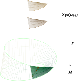
However, attempting to glue these together over all of $M$ runs into a problem: if we glue the two covers shown in this figure counterclockwise while respecting orientation, then upon returning to $x$, $(x,+)$ and $(x,-)$ are interchanged, so we must cross-glue the upper and lower components. The resulting double cover of $M$ is homeomorphic to a cylinder.

By definition, for $M$ to be orientable, there must exist a global section of $\omega_M$, which is equivalent to $\Spe(\omega_M)$ being a trivial covering space, which in turn is equivalent to $\omega_M$ being a constant sheaf. Applying §Covering Spaces, ⁋Corollary 12 (Fundamental theorem of covering spaces, classical version), we obtain the following proposition.

Proposition 6 For a (connected) topological manifold $M$, the following are equivalent.

$M$ is orientable.
$\Spe(\omega_M)$ has two components.
The monodromy action of $\pi_1(M)$ acts trivially on $\Spe(\omega_M)$.

However, since when dealing with homology and cohomology we have already extended not only to $\mathbb{Z}$-modules but also to general $A$-modules, the above argument can also be extended to a general $A$-module. To this end, if we first consider the relative homology version of §Cohomology, ⁋Proposition 1 (Universal coefficient theorem for homology), let us observe that the following (non-canonical) isomorphism

\[H_k(M, M\setminus\{x\};A)\cong H_k(M,M\setminus\{x\})\otimes_\mathbb{Z}A\oplus\Tor_1^\mathbb{Z}(H_{k-1}(M, M\setminus\{x\}), A)\]

exists. Now, since $H_k(M,M\setminus \{x\})$ is always a trivial group when $k\neq m$, from this isomorphism we know that

\[H_m(M,M\setminus \{x\};A)\cong H_m(M,M\setminus\{x\})\otimes_\mathbb{Z}A\cong A\]

Therefore, replacing every occurrence of $\mathbb{Z}$ in the above argument with $A$ will also make sense, and in particular we will obtain the presheaf of $A$-orientations

\[\omega_M^A(U)=\prod_{x\in U}\Iso_A(H_m(M,M\setminus\{x\};A), \underline{A}_x)\]

and the notion of a global $A$-orientation defined from it. The resulting $A$-orientation sheaf $\omega_M^A$ is nothing other than the subsheaf of $\or_M\otimes A$ collecting only the $A^\times$ of each stalk.

To derive a result like Proposition 6 from this definition, let us revisit §Covering Spaces, ⁋Theorem 11 (Fundamental theorem of covering spaces). For each covering space $p:E \rightarrow M$, we considered the $\pi_1(M,x)$-action on the fiber $p^{-1}(x)$ defined by the monodromy functor, which was the same as considering a group homomorphism $\pi_1(M,x)\rightarrow \Aut(p^{-1}(x))$. Then, for the covering space $p:\Spe(\omega_M)\rightarrow M$, we must examine how the $\pi_1(M,x)$-action is defined; here, the fiber $p^{-1}(x)$ is defined from the automorphisms of the stalk $\mathbb{Z}$,

\[\Iso_\mathbb{Z}(\mathbb{Z},\mathbb{Z})\cong \mathbb{Z}^\times\cong \{\pm 1\}\]

and therefore the $\pi_1(M,x)$-action can be thought of precisely as a group homomorphism $\pi_1(M,x)\rightarrow \mathbb{Z}^\times$. Then, since an $A$-module isomorphism from $A$ to $A$ corresponds exactly to an element of the unit group $A^\times$ of $A$, this consequently amounts to examining a group homomorphism $\pi_1(M,x)\rightarrow A^\times$. That is, Proposition 6 can be generalized as follows.

Proposition 7 For a (connected) topological manifold $M$, the following are equivalent.

$M$ is $A$-orientable.
$\Spe(\omega_M^A)$ is the trivial covering $M\times \lvert A^\times\rvert$.
The monodromy representation $\pi_1(M)\rightarrow A^\times$ is trivial.

The most notable case of this generalization is when $A=\mathbb{Z}/2$. In this case, the only unit of $A$ is $-1=1$, so the method of specifying an orientation is unique, and hence any manifold is always $\mathbb{Z}/2$-orientable.

Fundamental Class

We now examine the existence of a global ($A$-)orientation. That is, given, for all $x\in M$, local orientations $s_x$, we will examine whether there exists a suitable global section $s:M\rightarrow \Spe(\omega_M^A)$ such that $s(x)=(x,s_x)$.

Meanwhile, we know that via the canonical homomorphism

\[H_m(M; A)\rightarrow H_m(M,M\setminus\{x\};A)\tag{2}\]

any top homology class $\alpha\in H_m(M;A)$ defines an element $\alpha_x\in H_m(M,M\setminus\{x\};A)$ of the local homology group. Then one natural question would be whether, viewing for each $x\in M$ the given local orientations $s_x$ as elements of $A^\times$ and treating them as elements of $H_m(M,M\setminus\{x\};A)$, there exists, such that for all $x\in M$ the image of $\alpha\in H_m(M;A)$ in $H_m(M,M\setminus\{x\};A)$ is $s_x$, an $\alpha$.

The two paragraphs above illustrate what form Poincaré duality takes. A global section $s:M \rightarrow \Spe(\omega_M^A)$ is essentially a function defined over all of $M$, corresponding to the notion of $0$th cohomology. On the other hand, $\alpha\in H_m(M;A)$ is an element of $m$th homology. Poincaré duality shows that these two notions are equivalent and, more generally, shows the duality between $k$th cohomology and $m-k$th homology.

Now in the remainder of this post, there are broadly two things we must do.

Show that a lifting of the canonical homomorphism (2) defines a global orientation, and that the converse also holds.
Define the language of sheaf cohomology that can express the existence of a global orientation $M \rightarrow \Spe(\omega_M^A)$.

The core content of Poincaré duality is all contained in the first step, and the second step is closer to learning a language that expresses this elegantly. Therefore, we first begin with the first step. This is obtained by the following lemma.

Lemma 8 Fix a topological manifold $M$ of dimension $m$. In $M$, for any compact subset $C$, the following hold.

Given any section $s:M \rightarrow \Spe(\omega_M^A)$, there exists a unique homology class
\[\alpha_C\in H_m(M,M\setminus C;A)\]
such that for every $x\in C$, under the canonical homomorphism
\[H_m(M,M\setminus C;A)\rightarrow H_m(M,M\setminus\{x\};A)\]
the image of $\alpha_C$ is $s_x$.
For all $i>m$, we have $H_i(M, M\setminus C;A)=0$.

Proof

First, we show that if the statement holds for arbitrary compact sets $C_1,C_2$ and their intersection $C_1\cap C_2$, then it also holds for $C_1\cup C_2$. This is because in the Mayer–Vietoris sequence

\[\cdots \rightarrow H_k(M,M\setminus (C_1\cup C_2); A)\rightarrow H_k(M,M\setminus C_1;A)\oplus H_k(M,M\setminus C_2;A)\rightarrow H_k(M, M\setminus (C_1\cap C_2);A)\rightarrow\cdots\tag{3}\]

for $k>m$, by the inductive hypothesis

\[H_k(M,M\setminus C_1;A)=H_k(M,M\setminus C_2;A)=H_k(M,M\setminus(C_1\cap C_2);A)=0\]

so $H_k(M,M\setminus (C_1\cup C_2);A)$ must also be $0$, from which the second claim follows.

To prove the first claim, suppose a section $s:M \rightarrow \Spe(\omega_M^A)$ is given. By the inductive hypothesis, these admit liftings for $C_1,C_2,C_1\cap C_2$, so we must glue them together to produce a class $\alpha_{C_1\cup C_2}$ for $C_1\cup C_2$. By the uniqueness of these $\alpha_{C_1},\alpha_{C_2},\alpha_{C_1\cap C_2}$, both $\alpha_{C_1}$ and $\alpha_{C_2}$ must become the same element in $\alpha_{C_1\cap C_2}$; hence, considering the element

\[(\alpha_{C_1},-\alpha_{C_2})\in H_m(M,M\setminus C_1;A)\oplus H_m(M,M\setminus C_2;A)\]

in (3), this element belongs to the kernel of $H_m(M,M\setminus C_1;A)\oplus H_m(M,M\setminus C_2;A)\rightarrow H_m(M, M\setminus (C_1\cap C_2);A)$, and therefore we can choose an element of $H_m(M,M\setminus (C_1\cup C_2);A)$; uniqueness follows from the injectivity of

\[0=H_{m+1}(M,M\setminus (C_1\cap C_2);A)\rightarrow H_m(M,M\setminus (C_1\cup C_2);A)\rightarrow H_m(M,M\setminus C_1;A)\oplus H_m(M,M\setminus C_2;A)\]

Now, for the base case of the induction, it suffices to consider the case where $M=\mathbb{R}^m$ and $C$ is a convex compact subset. This is because after covering a compact set of an arbitrary manifold $M$ by Euclidean charts and using compactness, it suffices to assume $M=\mathbb{R}^m$, and inside $\mathbb{R}^m$ it is enough to look only at sets containing $C$ that are finite unions $K$ of closed balls. For the maps given by the inclusion relation $\mathbb{R}^m\setminus K\subseteq\mathbb{R}^m\setminus C$,

\[\varinjlim_{K\supseteq C}H_i(\mathbb{R}^m,\mathbb{R}^m\setminus K;A)\cong H_i(\mathbb{R}^m,\mathbb{R}^m\setminus C;A)\]

holds. Indeed, this map consists of those induced by the inclusion $\mathbb{R}^m\setminus K\hookrightarrow \mathbb{R}^m\setminus C$, that is, $C\hookrightarrow K$, and therefore for this to be an isomorphism, the map induced by each $C\hookrightarrow K$ must be an isomorphism. By definition, singular chains are always compact, so this always holds. Then, in this base case, both spaces $\mathbb{R}^m\setminus C$ and $\mathbb{R}^m\setminus \{x\}$ deformation retract to the same space $S^{m-1}$, so it is an isomorphism, and from this the proof is complete.

In this proof, compactness is essential for this inductive process to terminate in finitely many steps when constructing $\alpha$ inductively using the Mayer–Vietoris sequence. In fact, if compactness is dropped, Poincaré duality takes a somewhat different form, and what must be introduced to express it in a unified formula is the language of sheaf cohomology.

At any rate, by Lemma 8 above, if $M$ is a compact topological manifold of dimension $m$, then setting $C=M$ yields the following theorem.

Theorem 9 Let $M$ be a compact connected topological manifold of dimension $m$. Then for every global orientation $s:M \rightarrow \Spe(\omega_M^A)$, there exists a unique class $[M]\in H_m(M;A)$ such that the image of $[M]$ under the canonical homomorphism (2) coincides with $s_x$.

Then by Lemma 8, $H_m(M;A)$ is generated by $[M]$ as a free $A$-module of rank 1, and different choices of global orientation correspond to different choices of generators of $H_m(M;A)$.

Definition 10 We call the class $[M]$ defined in Theorem 9 above, defined by the global orientation $s$, the fundamental class of $M$.

Moreover, if a homology class $[M]$ satisfying the condition of Theorem 9 exists, we know that a global section $s:M \rightarrow \Spe(\omega_M^A)$ is given from this.

Poincaré Duality

We can now prove Poincaré’s theorem when the given manifold is $A$-orientable. To this end, consider the following cap product homomorphism:

\[-\frown -: H^p(M;A)\otimes_A H_m(M;A) \rightarrow H_{m-p}(M;A)\]

Then, since $H_m(M;A)\cong A$, this homomorphism from $H^p(M;A)$ to $H_{m-p}(M;A)$ may be regarded as an $A$-module homomorphism. In particular, introducing a generator of $H_m(M;A)$, $[M]$, this becomes the following homomorphism:

\[-\frown [M]: H^p(M;A)\rightarrow H_{m-p}(M;A)\]

Theorem 11 For an $A$-orientable compact manifold $M$ of dimension $m$ and its fundamental class $[M]$, the above homomorphism

\[-\frown [M]: H^p(M;A)\rightarrow H_{m-p}(M;A)\]

is an isomorphism.

The proof of this also proceeds by induction using the Mayer–Vietoris sequence, just as in the proof of Lemma 8. The somewhat different point, however, is that in Lemma 8 the assertion was about a compact subset $C$, so compactness could be actively used, whereas this time the assertion is about $M$ itself; thus, for instance, if for $M$ a chart $U$ is given, this is not compact, so one cannot approach this by simple induction. For this, we define the following.

Definition 12 A cochain $\varphi\in C^p(M;A)$ is said to be compactly supported if there exists a compact set $K\subseteq M$ such that $\varphi(\sigma)=0$ holds for every simplex lying in $M\setminus K$. The $p$-th cohomology of the cochain complex of compactly supported cochains is called the $p$-th compactly supported cohomology, and is denoted by $H_c^p(M;A)$.

Then the identity

\[H_c^p(M;A)\cong \varinjlim_{\text{\scriptsize$K$ compact}}H^p(M,M\setminus K;A)\]

holds. For each compact set $K$, the canonical map

\[H^p(M,M\setminus K;A)\rightarrow H_c^p(M;A)\]

exists, and it is compatible with the directed system on the right-hand side, so the homomorphism

\[\varinjlim_{\text{\scriptsize$K$ compact}}H^p(M,M\setminus K;A)\rightarrow H_c^p(M;A)\]

is well defined. That this is actually an isomorphism can be checked at the cochain level. Intuitively, the $K$’s are the supports of the cochains, and since a finite union of compact sets is again compact, their collection forms a directed system; taking the direct limit, that is, the union, is an exact functor, and so it commutes with taking cohomology. In particular, for any compact manifold $M$, we have $H_c^p(M;A)\cong H^p(M;A)$, and therefore the desired result follows from the next lemma.

Lemma 13 For any $A$-orientable $m$-manifold $M$, the isomorphism

\[H_c^p(M;A)\cong H_{m-p}(M;A)\]

holds for all $p$.

Proof

To this end, we must first define the isomorphism. For this, for any compact subset $K$, consider the cap product

\[H^p(M,M\setminus K;A)\times H_m(M,M\setminus K;A)\rightarrow H_{m-p}(M;A)\]

Then by Lemma 8, we can find, agreeing upon restriction to each point $x$ with the orientation of $M$, $s_x$, a homology class

\[s_K\in H_m(M,M\setminus K;A)\]

Our claim is that the cap product homomorphism constructed from these $s_K$,

\[-\frown s_K: H^p(M,M\setminus K;A) \rightarrow H_{m-p}(M;A)\]

satisfies compatibility for the direct system, and therefore defines a homomorphism $H_c^p(M;A)\rightarrow H_{m-p}(M;A)$. To verify this, suppose $K$ is contained in another compact subset $K'$, and the inclusion $i:K\rightarrow K'$ is given. Then for any $\alpha\in H^p(M,M\setminus K;A)$,

\[i^\ast\alpha\frown s_{K'}=\alpha\frown i_\ast s_{K'}\]

holds by §Cup Product, ⁋Proposition 6 (Projection formula), and by the uniqueness in Lemma 8 we have $i_\ast s_{K'}=s_K$, so we see that this well-defines the homomorphism $H_c^p(M;A)\rightarrow H_{m-p}(M;A)$.

Our claim is that this homomorphism $D_M:H_c^p(M;A)\rightarrow H_{m-p}(M;A)$ is an isomorphism, and to show this we use induction via the Mayer–Vietoris sequence, just as in the proof of Lemma 8.

The base step of the induction is the case $M=\mathbb{R}^m$. In this case, we know that for any ball $B\subseteq \mathbb{R}^m$, the orientation of $B$, $s_B$, gives

\[H_m(\mathbb{R}^m, \mathbb{R}^m\setminus B;A)\cong A\]

and from §Cohomology, ⁋Proposition 3 (Universal coefficient theorem for cohomology), $H^m(\mathbb{R}^m,\mathbb{R}^m\setminus B;A)\cong A$; here, corresponding to the dual basis of the orientation of $B$, the element $\alpha_B$ satisfies the equation

\[\langle 1\smile \alpha_B, s_B\rangle=\langle 1,\alpha_B\frown s_B\rangle\]

so we know that $\alpha_B\frown s_B$ corresponds to a generator of $H_0(\mathbb{R}^m)\cong A$, and therefore

\[H^p(\mathbb{R}^m,\mathbb{R}^m\setminus B;A)\cong H_{m-p}(\mathbb{R}^m;A)\]

holds for all $p$. (The case $p\neq m$ is an isomorphism because it is the zero map between zero modules.) Now, forming a directed system covering all of $\mathbb{R}^m$ by increasing the radius of $B$, we see that $H_c^p(M)\rightarrow H_{m-p}(M)$ is an isomorphism.

Now as the next step, suppose $M$ has two open subsets $U,V$ such that $M=U\cup V$ and the given proposition holds for $U,V,U\cap V$. Then for each compact subset $K\subseteq U$, $L\subseteq V$, considering the relative Mayer–Vietoris sequence

\[\cdots\rightarrow H^k(M,M\setminus(K\cap L);A)\rightarrow H^k(M,M\setminus K;A)\oplus H^k(M,M\setminus L;A)\rightarrow H^k(M,M\setminus(K\cup L);A)\rightarrow \cdots\]

and then applying excision and taking the limit, we obtain the following diagram

This diagram may have a sign discrepancy in the square involving the connecting homomorphism and is therefore commutative only when signs are ignored; however, signs are not needed to apply [Homological Algebra] §Diagram chasing, ⁋Corollary 2 (The five lemma), so together with the inductive step, the induction is completed.

However, since there is no assumption that $M$ is compact, a little extra argument must be added. First, suppose $M$ is the union of a nested family of open subsets

\[U_1\subseteq U_2\subseteq\cdots\]

and that the given proposition holds for each of them. Then any compact subset of $M$ must be contained in some $U_i$, from which we obtain the following isomorphisms

\[H_c^p(M)=\varinjlim_i H^p_c(U_i),\qquad H_{m-p}(M)=\varinjlim_i H_{m-p}(U_i)\]

Since by assumption all $H^p_c(U_i)\rightarrow H_{m-p}(U_i)$ are isomorphisms, we obtain the desired result.

Now consider the case where $M$ is an open subset of $\mathbb{R}^m$. Then we can first cover $M$ by countably many convex open subsets (i.e. open balls) homeomorphic to $\mathbb{R}^m$, $U_1,U_2,\ldots$, and since any convex open subset is homeomorphic to $\mathbb{R}^m$, we saw in the base step above that the theorem’s isomorphism holds for each of them. Also, since the intersection of two convex sets is again convex, by the induction above the conclusion holds for $U_1\cup U_2$ as well. Next, in order to show that the conclusion holds for $U_1\cup U_2\cup U_3$, we must show that the following intersection

\[(U_1\cup U_2)\cap U_3=(U_1\cap U_3)\cup (U_2\cap U_3)\]

satisfies the given condition; here we know that $U_1\cap U_3$, $U_2\cap U_3$, and $U_1\cap U_2\cap U_3$ all satisfy the given condition as convex open subsets of $\mathbb{R}^m$. In a similar manner, we know that each of

\[U_1,\quad U_1\cup U_2, \quad U_1\cup U_2\cup U_3,\quad \cdots\]

satisfies the conclusion. Therefore, applying the preceding (infinite) induction to the sequence of nested open subsets

\[U_1\subseteq U_1\cup U_2\subseteq U_1\cup U_2\cup U_3\cdots\]

yields the desired result.

Now finally, if $M$ is an arbitrary manifold, using second countability we may cover $M$ by countably many Euclidean charts and repeat the same argument as above.

In particular, in the proof, if $M$ itself were compact, the duality map $D_M$ would have been precisely the cap product with the fundamental class $[M]$.

Twisted Poincaré Duality

When $M$ is not $A$-orientable, the primary reason Theorem 11 fails to hold is that, fundamentally, $\omega_M^A$ fails to be a constant sheaf and is merely locally constant. In the language of covering spaces, this can be understood as saying that because the monodromy action acts nontrivially on the stalk $A$, after going “once around” the stalk $A$ is glued with a twist. Since this twist is an automorphism of $A$, to see this, it was sufficient for us to consider elements of the unit group of $A$, $A^\times$.

Now, in order to take this twist into account in duality, we define homology with local coefficients.

Definition 14 A locally constant sheaf $\mathcal{L}$ defined on $M$ is called a local coefficient system.

Let $L$ be the stalk of a local system $\mathcal{L}$. Then by §Covering Spaces, ⁋Theorem 11 (Fundamental theorem of covering spaces), we know that whenever a path $\alpha:[0,1]\rightarrow M$ is given, there exists an isomorphism $\mathcal{L}_{\alpha(0)}\rightarrow \mathcal{L}_{\alpha(1)}$ between stalks. This is nothing other than the isomorphism obtained by lifting the path $\alpha$ in the covering space $\Spe(\mathcal{L})\rightarrow M$. That is, we obtain the following functor

\[\Pi_1(M)\rightarrow \Ab; \qquad x\mapsto \mathcal{L}_x\]

Then fixing a point $e_0=(1,0,\ldots,0)$ of $\Delta^k$, we define $C_\bullet(M,\mathcal{L})$ by the formula

\[C_k(M,\mathcal{L})=\bigoplus_{\sigma:\Delta^k\rightarrow M}\mathcal{L}_{\sigma(e_0)}\]

In any case, $\mathcal{L}_x\cong L$ for each $x$, but the key point of this definition is that $L$ at each point may differ via a nontrivial automorphism. Then the differential map of this chain complex is defined, for a singular $k$-simplex $\sigma:\Delta^k \rightarrow M$ and a coefficient $a\in \mathcal{L}_{\sigma(e_0)}$, by

\[\partial_k(a\sigma)=\sum_{i=0}^k(-1)^i\mathcal{L}_{\sigma_i}(a) (\sigma\vert_{[v_0,\ldots, \hat{v}_i,\ldots,v_k]})\]

Here $\mathcal{L}_{\sigma_i}$ is obtained by applying the functor $\Pi_1(M) \rightarrow \Ab$ to the path obtained by sending the edge joining the first vertex $\sigma(e_0)$ of the original simplex and the first vertex of the $i$-th face into $M$. In nice situations like ours, we know that even if we consider the chain complex obtained by constructing

\[C(\widetilde{M})\otimes_{\mathbb{Z}[\pi_1(M)]} L\]

using the universal cover $\widetilde{M}$ of $M$, the monodromy action (i.e., Deck transformation) acting on it, and the monodromy representation $\pi_1(M)\rightarrow \Aut(L)$, this gives the same homology group as the one above.

In a sense, this might be seen as a somewhat excessive generalization, because to describe the non-orientable version of Poincaré duality we will anyway set the local coefficient system $\mathcal{L}$ to be the constant sheaf $\underline{A}$. However, through this generalization we can also generalize the cohomology part, and this generalization makes Poincaré duality somewhat more transparent.

For any topological space $X$ and a sheaf $\mathcal{F}$ defined on it, the global section functor

\[\Gamma(X,-):\Sh(X;\mathcal{A})\rightarrow \mathcal{A}\]

is a left exact functor, so its right derived functors exist. To compute these directly, we use the Godement resolution, which is defined as follows.

Consider a topological space $X$ and a sheaf $\mathcal{F}$ defined on it, and consider the étalé space $\Spe(\mathcal{F})$. We know that $\mathcal{F}$ is precisely the sheaf of continuous sections of $\Spe(\mathcal{F})\rightarrow X$. Now for any open set $U$, let us define

\[\mathcal{G}_0(U)=\prod_{x\in U}\mathcal{F}_x\]

That is, $\mathcal{G}_0$ is the sheaf of (not necessarily continuous) set-theoretic sections of $\Spe(\mathcal{F})\rightarrow X$. Our idea is to push into the quotient sheaf $\mathcal{Q}$, through the following sequence

\[0 \rightarrow \mathcal{F}\rightarrow \mathcal{G}_0 \rightarrow \mathcal{Q}\rightarrow 0\]

induced by the inclusion $\mathcal{F}\rightarrow \mathcal{G}_0$, the cases where locally defined functions in general fail to become a function when glued together. Then for the sheaf $\mathcal{Q}$ as well, we can similarly construct a sheaf defined by

\[\mathcal{G}_1(U)=\prod_{x\in U}\mathcal{Q}_x\]

and this defines the following Godement resolution

\[0 \rightarrow \mathcal{F}\rightarrow \mathcal{G}_0 \rightarrow \mathcal{G}_1\rightarrow \cdots\]

Intuitively, this repeatedly places the part preventing $\Spe(\mathcal{F})$ from having a global section into $\mathcal{Q}$, and then again the part preventing $\mathcal{Q}$ from having a global section into $\mathcal{Q}'$, and so on. This resolution $\mathcal{G}_\bullet$ is not an injective resolution, but because each sheaf is a flabby (flasque) sheaf, we can compute the right derived functors $R^i\Gamma$ of the global section functor through it.

Definition 15 For a topological space $X$ and a sheaf $\mathcal{F}$ defined on it, the $k$-th cohomology of the sequence of global sections of the Godement resolution

\[0 \rightarrow \mathcal{G}_0(X)\rightarrow \mathcal{G}_1(X)\rightarrow \cdots\]

is denoted by

\[H^k(X; \mathcal{F})\]

and is called sheaf cohomology.

This is treated in more detail in [Algebraic Varieties] §Sheaf Cohomology, ⁋Definition 1. Now if $M$ is compact, Poincaré duality generalizes to the following isomorphism:

\[H^k(M;\mathcal{L})\cong H_{m-k}(M;\omega_M^A\otimes \mathcal{L})\]

Here, to return to the original Poincaré duality, we first set $\mathcal{L}$ to be the constant sheaf $\underline{A}$. Then, in nice cases such as manifolds, it is known that the sheaf cohomology $H^k(M;\underline{A})$ and the singular cohomology $H^k(M;A)$ are isomorphic, so we obtain the following isomorphism:

\[H^k(M;A)\cong H_{m-k}(M;\omega_M^A)\]

Furthermore, if $M$ is $A$-orientable, then $\omega_M^A$ also becomes a constant sheaf, and from this we can recover the classical Poincaré duality:

\[H^k(M;A)\cong H_{m-k}(M;A)\]

Poincaré Duality and Cup Product

So far we have used the cup product on the cohomology ring and the cap product defined from it without hesitation. However, if someone were to ask what the cup product is, it would be difficult to answer. The answer to this is simple.

The cup product is the Poincaré dual of intersection.

To explain rigorously what this means would require at least as much additional effort as we have invested so far. However, to see intuitively what this means, the following example will probably suffice.

Example 16 Consider the torus $T^2=S^1\times S^1$. Then from the Künneth formula we know that the cohomology of $T^2$ is

\[H^0(T^2;\mathbb{Z})\cong \mathbb{Z}, \quad H^1(T^2;\mathbb{Z})\cong \mathbb{Z}^2,\quad H^2(T^2;\mathbb{Z})\cong \mathbb{Z}\]

In this cohomology ring, the only non-trivial product is the product of the two generators of $H^1(T^2;\mathbb{Z})$, $\alpha,\beta$. By §Cohomology, ⁋Proposition 3 (Universal coefficient theorem for cohomology), these correspond to the duals of the two circles of $T^2$. Then taking their cup product gives a generator of $H^2(T^2;\mathbb{Z})$, which is obtained directly from the definition of the cup product, or algebraically obvious since

\[H^2(T^2;\mathbb{Z})=H^1(S^1;\mathbb{Z})\otimes H^1(S^1;\mathbb{Z})\cong \mathbb{Z}\otimes \mathbb{Z}\cong \mathbb{Z}\]

is generated by $\alpha\otimes \beta$.

Here, the reason their cup product does not appear as a constant multiple of $\alpha\times \beta$ other than $\pm 1$ is geometrically as follows. If we let the homology classes corresponding to $\alpha$ and $\beta$ be $a,b$, this is because the intersection of $a$ and $b$ meets at only one point, as shown in the following figure.

$Torus_intersection$

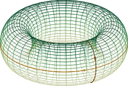
Here, classifying how the two curves meet and assigning one as the positive direction and the other as the negative direction is the same as giving an orientation of $T^2$.

Then under this geometric interpretation, how can we explain that $\alpha^2=0$? If we compute the intersection $a\cap a$ literally, this becomes $a$ again. The reason this computation gets tangled is that the two cycles (in this case, two copies of $a$) are not in general position. Roughly, given any two lines in $\mathbb{R}^2$, they will generally meet at one point (except when they are parallel, including the coincident case), and the notion of general position generalizes this.

Now consider curves of homology class $a$ on $T^2$. Then they will most likely not meet each other, and if they do (again excluding the non-general position case of tangency), they will meet in the following shape

At first glance this seems to produce two intersection points, but in the figure above the two intersections have opposite signs; that is, for example, taking the line as the first vector and the curve as the second vector and computing the cross product, one will give a vector pointing outward and the other a vector pointing inward, so the signs are opposite. Thus the two intersection points cancel and their intersection becomes $0$, and therefore $\alpha\smile\alpha=0$.

References

[Hat] A. Hatcher, Algebraic Topology. Cambridge University Press, 2022.
[May] J. P. May, A concise course in algebraic topology.

K

Poincaré Duality

Orientation Sheaf

Constant Sheaves, Covering Spaces, and Orientation-Generator Sheaves

Fundamental Class

Poincaré Duality

Twisted Poincaré Duality

Poincaré Duality and Cup Product

Share on

Comments

Leave a comment

찾아보기