Rational Maps

This post was machine-translated from the Korean original by Marvin (via Kimi). It may contain errors or awkward phrasing — the Korean original is the source of truth.

In §Quasi-Projective Varieties, ⁋Definition 7 we defined regular maps between quasi-projective varieties. Above all, these are functions defined at every point of the domain; even if they are written in rational form on \(D(f)\) as in §Affine Varieties, ⁋Definition 14, the only denominators allowed are powers of \(f\), so they are defined everywhere.

Nevertheless, many kinds of functions are given in forms that are not regular maps. For example, \((x, y) \mapsto [x : y]\) is not a regular map because it is undefined at the origin, yet it looks like a perfectly natural function. In this post we study rational maps, which are functions defined at most points.

Rational Functions

Just as when we defined regular maps, we first define the notion of a rational function before defining rational maps.

Definition 1 A rational function on a variety \(X\) is a pair \((U,f)\) consisting of a nonempty open subset \(U\) of \(X\) and a regular function \(f:U \rightarrow \mathbb{K}\) defined on it. Two rational functions \((U,f)\) and \((V,g)\) are equivalent if they agree on \(U\cap V\).

The intuition is as follows. In the Zariski topology closed sets are small and open sets are large. Thus a rational function is a function that fails to be defined on a small set but is defined at most of the remaining points. For instance, one may essentially think of open sets in the Zariski topology as being of the form \(D(g)\), and the regular functions \(f/g\) defined on them are now regarded as functions. (§Affine Varieties, ⁋Definition 14) Of course this function is undefined where \(g=0\), but that is precisely why we consider functions defined on an open set \(U\), and in any case the points where \(g=0\) are small when viewed in the whole space.

We denote the set of all rational functions on \(X\) by \(\mathbb{K}(X)\). The sum and product of two rational functions are defined on the intersection of their domains of definition, and the inverse of a nonzero rational function is defined at the points where that function is nonzero. Hence \(\mathbb{K}(X)\) is a field, which we call the function field.

Proposition 2 For an affine variety \(X\), we have \(\mathbb{K}(X)=\Frac\mathbb{K}[X]\).

The essential part of this proposition is to represent an arbitrary regular function \(f:U\rightarrow \mathbb{K}\) defined on an arbitrary open set \(U\) actually in fractional form; but since \(U\) can be expressed as a union of \(D(f)\)’s (§Affine Varieties, ⁋Proposition 6) and the regular functions on it are of the form of rational expressions with powers of \(f\) in the denominator, the proof is not difficult.

What is important is that this proposition provides a practical way to compute rational functions. For example, for \(X = V(\y - \x^2)\) the coordinate ring is \(\mathbb{K}[\x, \y]/(\y - \x^2) \cong \mathbb{K}[\x]\), and hence \(\mathbb{K}(X) = \operatorname{Frac}(\mathbb{K}[\x]) = \mathbb{K}(\x)\).

Proposition 3 For a variety \(X\) and a nonempty open subset \(U\), we have \(\mathbb{K}(U) = \mathbb{K}(X)\).

Proof

First, it is obvious that the inclusion \(\iota: U \hookrightarrow X\) induces an embedding \(\iota^\ast: \mathbb{K}(X)\rightarrow \mathbb{K}(U)\) of function fields. Since any nonzero field homomorphism is an inclusion, it suffices to show that \(\iota^\ast\) is surjective. (§Fields, ⁋Proposition 2)

Now for any \(f \in \mathbb{K}(U)\), \(f\) is a regular function on some nonempty open subset \(V\) of \(U\), and then since this \(V\) is also an open subset of \(X\), the pair \((V,f)\) belongs to \(\mathbb{K}(X)\).

Example 4 Considering the function field \(\mathbb{K}(\mathbb{P}^n)\) of \(\mathbb{P}^n\), by Proposition 3 it suffices to compute the function field on the open set \(U_0\) of \(\mathbb{P}^n\). But \(U_0\) is an affine variety, so by Proposition 2 it equals the fraction field of \(\mathbb{K}[U_0]\), and therefore the function field of \(\mathbb{P}^n\) is the field \(\mathbb{K}(\t_1,\ldots, \t_n)\) generated by \(n\) indeterminates.

Concretely, this is obtained by expressing an element of \(\mathbb{P}^n\) as \([x_0:\cdots: x_n]\) and setting \(\t_i=\x_i/\x_0\) where \(\x_i\) is the coordinate function reading off the \(i\)-th coordinate. If we had chosen a different open set \(U_j\), similar rational functions would have been defined via \(\t_i=\x_i/\x_j\), and hence we know in general that rational functions on \(\mathbb{P}^n\) are represented in the form \(F/G\), the ratio of homogeneous polynomials of the same degree.

Rational Maps

Now, thinking about how we defined regular maps from regular functions, it is obvious how to define rational maps from rational functions.

Definition 5 A rational map between two varieties \(X, Y\) is a pair \((U,\varphi)\) consisting of a nonempty open subset \(U\) of \(X\) and a regular map \(\varphi: U \to Y\) defined on it.

As before, two rational maps \(\varphi: U \to Y\) and \(\psi: V \to Y\) are regarded as the same if they agree on \(U \cap V\). A rational map is usually denoted \(\varphi: X \dashrightarrow Y\), where the dashed arrow indicates that it may not be defined at every point. The points where it is undefined are called base points.

On the other hand, for a rational map \(\varphi:U\rightarrow Y\) we can consider rational functions equivalent to \((U,\varphi)\). Then taking the union of the domains of all these rational functions, we obtain the largest open set on which \(\varphi\) can be defined.

Definition 6 For a rational map \(\varphi: X\dashrightarrow Y\), we denote by \(\dom(\varphi)\) the open set obtained by the above procedure.

Example 7 One of the typical examples of a rational map is the projection from a point. For instance, considering the line \(\{\x_2=0\}\) in \(\mathbb{P}^2\), we may think of this as a projective line \(\mathbb{P}^1\) inside \(\mathbb{P}^2\). Now the point \([0:0:1]\) does not lie on this line, and the equation of the line joining this point and an arbitrary point \([x_0:x_1:x_2]\) is

\[x_1\x_0-x_0\x_1=0\]

Then the point where this line meets the above \(\mathbb{P}^1\) is exactly \([x_0:x_1:0]\), and hence the following projection

\[[x_0:x_1:x_2]\mapsto [x_0:x_1]\]

is obtained through this projection.

Birational Equivalence

If an isomorphism of regular maps means that two varieties have exactly the same structure, then birational equivalence means that two varieties have essentially the same structure. Many geometric properties are preserved not only between isomorphic varieties but also between birationally equivalent varieties.

Definition 8 A rational map \(\varphi: X \dashrightarrow Y\) is said to be dominant if its image is dense in \(Y\). That is, \(\overline{\varphi(X)} = Y\) holds.

Definition 9 A rational map \(\varphi: X \dashrightarrow Y\) is a birational map if there exists another rational map \(\psi: Y \dashrightarrow X\) such that \(\psi \circ \varphi = \operatorname{id}_X\) and \(\varphi \circ \psi = \operatorname{id}_Y\) hold (where defined). Two varieties \(X, Y\) are said to be birationally equivalent if there exists a birational map between them.

Two birationally equivalent varieties are isomorphic “at most points.” Concretely, as we see in the following proposition, there exist isomorphic open subsets of the two varieties. This shows that birational equivalence is weaker than isomorphism but still a strong relationship.

Proposition 10 For two varieties \(X, Y\) the following are equivalent.

1. \(X\) and \(Y\) are birationally equivalent.
2. \(\mathbb{K}(X) \cong \mathbb{K}(Y)\) holds.
3. There exist nonempty isomorphic open subsets of \(X\) and \(Y\).

Proof

First, suppose \(X, Y\) are birationally equivalent. Then considering the domain \(\dom(\varphi)\) of the birational map \(\varphi: X\dashrightarrow Y\), there exists a homomorphism \(\varphi^\ast: \mathbb{K}(Y)\rightarrow \mathbb{K}(\dom(\varphi))\) of function fields induced by \(\varphi\). Similarly, the birational inverse \(\psi: Y\dashrightarrow X\) of \(\varphi\) defines \(\psi^\ast: \mathbb{K}(X)\rightarrow \mathbb{K}(\dom(\psi))\). Now by Proposition 3 we have \(\mathbb{K}(\dom(\varphi))=\mathbb{K}(X)\) and \(\mathbb{K}(\dom(\psi))=\mathbb{K}(Y)\), so using this we see that \(\mathbb{K}(X)\cong \mathbb{K}(Y)\).

Now suppose a field isomorphism \(\Phi: \mathbb{K}(X) \rightarrow \mathbb{K}(Y)\) is given. For any affine open subset \(U \subseteq X\), the coordinate ring \(\mathbb{K}[U]\) is a finitely generated \(\mathbb{K}\)-subalgebra of \(\mathbb{K}(X)\). Now take an affine open subset \(V\subseteq Y\) such that the images of its generators under \(\phi\) are all regular, and through this we can define \(\Phi\vert_{\mathbb{K}[U]}:\mathbb{K}[U]\rightarrow \mathbb{K}[V]\). On the other hand, in a similar way we can take \(\Phi^{-1}\vert_{\mathbb{K}[V]}:\mathbb{K}[V]\rightarrow \mathbb{K}[U']\) using \(\Phi^{-1}\), and then \(U'\subset U\) holds. Now from the assumption that \(\Phi\) is an isomorphism we must have \(\mathbb{K}[U]=\mathbb{K}[U']\) and \(\mathbb{K}[U]\cong \mathbb{K}[V]\).

That the last condition implies the first is obvious by Proposition 3.

This theorem shows that to determine birational equivalence it suffices to look at the function field.

Example 11 Let us compute the function fields of \(\mathbb{P}^1 \times \mathbb{P}^1\) and of the quadric surface \(Q = V(\x\y - \z\w)\) in \(\mathbb{P}^3\).

First, for \(\mathbb{P}^1 \times \mathbb{P}^1\), by Proposition 3 it suffices to compute on the product open set \(U_0 \times U_0\) of each factor. The function field of the first factor \(\mathbb{P}^1\) is \(\mathbb{K}(\t_1)\) as we saw in Example 4, and similarly the second factor is \(\mathbb{K}(\t_2)\). Then through this we know that their function field is given as \(\mathbb{K}(\t_1,\t_2)\).

Now consider the quadric surface \(Q = V(\x\y - \z\w) \subset \mathbb{P}^3\). Similarly by Proposition 3 it suffices to compute on the affine patch \(\{\w \ne 0\}\). On this patch setting \(\x' = \x/\w\), \(\y' = \y/\w\), \(\z' = \z/\w\), the equation \(\x\y - \z\w = 0\) becomes \(\x'\y' - \z' = 0\). Hence \(\z' = \x'\y'\), and the coordinate ring of this patch is \(\mathbb{K}[\x', \y', \z']/(\x'\y' - \z') \cong \mathbb{K}[\x', \y']\). By Proposition 2 we have \(\mathbb{K}(Q) = \operatorname{Frac}(\mathbb{K}[\x', \y']) = \mathbb{K}(\x', \y') \cong \mathbb{K}(\t_1, \t_2)\).

Therefore since \(\mathbb{K}(\mathbb{P}^1 \times \mathbb{P}^1) \cong \mathbb{K}(Q) \cong \mathbb{K}(\t_1, \t_2)\), by Proposition 10 the two varieties are birationally equivalent. In fact, the image of the Segre embedding \(\mathbb{P}^1 \times \mathbb{P}^1 \to \mathbb{P}^3\), \(([x : y], [u : v]) \mapsto [xu : xv : yu : yv]\) discussed in §Projective Varieties, ⁋Example 16 is exactly \(V(\x\y - \z\w)\). That is, in this case the birational equivalence is actually an isomorphism. This example shows that birational equivalence is weaker than isomorphism but includes isomorphism.

Blow-up

A rational map has the limitation that it is undefined at base points. A representative tool for resolving this limitation is the blow-up. The motivation for this is the very first function we considered, \((x,y)\mapsto [x:y]\). This function takes a point \((x,y)\) in \(\mathbb{A}^2\) and gives the slope of the line joining this point and the origin \((0,0)\in \mathbb{A}^2\), and the reason this is undefined at the origin is that two distinct points are needed to define a line. In such a case, we would usually fix the origin \((0,0)\), take another point \((x,y)\) approaching \((0,0)\), and compute the limit, but in this case there are infinitely many directions approaching \((0,0)\) so the limit is not well defined.

The idea of blow-up is simple: record all directions approaching \((0,0)\) separately.

Example 12 Consider the following variety

\[\Bl_{(0,0)} \mathbb{A}^2 = \{((x, y), [u : v]) \in \mathbb{A}^2 \times \mathbb{P}^1 \mid xv = yu\}\]

This set is a closed subvariety of \(\mathbb{A}^2 \times \mathbb{P}^1\). The condition \(xv = yu\) means that the point \((x, y)\) and the line \([u : v]\) are in the same direction. That is,

• For a point \((x,y)\) in \(\mathbb{A}^2\) other than the origin, the condition \(xv=yu\) determines a unique point \([u:v]\) in \(\mathbb{P}^1\), and through this the point of \(\Bl_{(0,0)}\mathbb{A}^2\) is uniquely determined.
• At the origin \((0,0)\) of \(\mathbb{A}^2\), every point of \(\mathbb{P}^1\) is possible.

[Har1] p.29. Fig. 3.

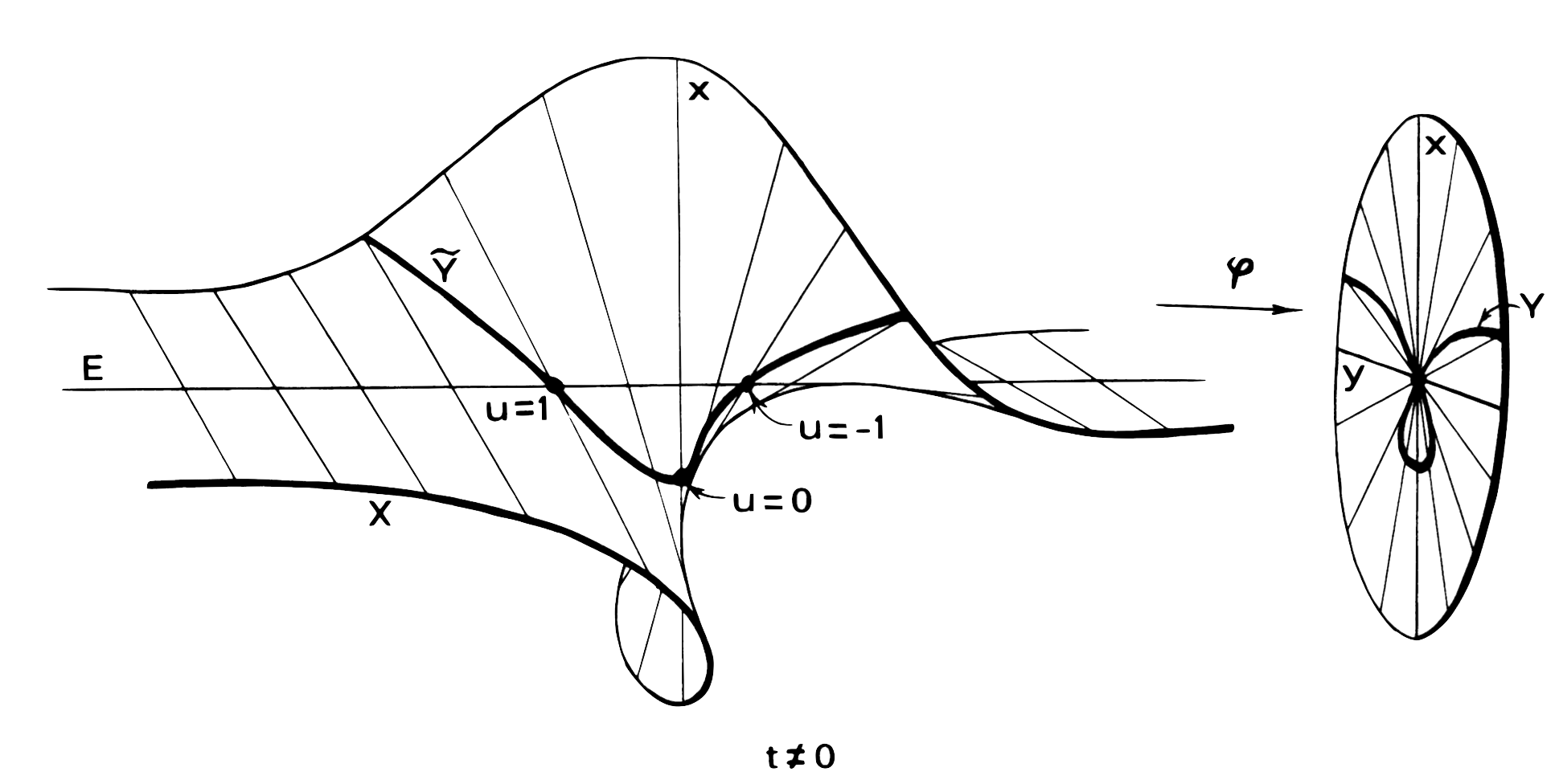
Concretely, defining the projection \(\pi_1: \operatorname{Bl}_{(0,0)} \mathbb{A}^2 \to \mathbb{A}^2\) by \(\pi((x, y), [u : v]) = (x, y)\), the preimage of every point other than the origin is a single point, and the preimage of the origin is \(\mathbb{P}^1\). This is called the exceptional divisor.

From this, since the two varieties \(\mathbb{A}^2\) and \(\Bl_{(0,0)}\mathbb{A}^2\) are isomorphic on the rest of the plane excluding the origin, \(\pi\) is a birational map.

Now consider the rational map \(\varphi: \mathbb{A}^2 \dashrightarrow \mathbb{P}^1\), \((x, y) \mapsto [x : y]\) mentioned earlier. This is undefined at the origin \((0, 0)\), but from the viewpoint of the blow-up \(\operatorname{Bl}_{(0,0)} \mathbb{A}^2\) it is simply the projection \(\pr_2\) to the \(\mathbb{P}^1\) factor, and in particular this is a regular map. In this way we can resolve base points at which a birational map is undefined.

---

References

[Har1] R. Hartshorne, Algebraic Geometry, Springer, 1977.
[Har2] J. Harris, Algebraic Geometry: A First Course, Springer, 1992.
[Sha] I. R. Shafarevich, Basic Algebraic Geometry I: Varieties in Projective Space, Springer, 2013.