Projective Varieties

This post was machine-translated from the Korean original by Marvin (via Kimi). It may contain errors or awkward phrasing — the Korean original is the source of truth.

Definition of Projective Space

We now define projective varieties, another important class of algebraic varieties. We begin with the following.

Definition 1 The projective \(n\)-space \(\mathbb{P}^n_{\mathbb{K}}\) over a field \(\mathbb{K}\) is defined as follows. As a set,

\[\mathbb{P}^n = (\mathbb{K}^{n+1} \setminus \{0\}) / \sim\]

where the equivalence relation \(\sim\) is given by

\[(x_0, \ldots, x_n) \sim (y_0, \ldots, y_n) \iff \text{$x_i = \lambda y_i$ for some $\lambda \in \mathbb{K}^\ast$, for all $i$}\]

We write \(\mathbb{P}^n\) when there is no risk of confusion.

The equivalence class \([(x_0, \ldots, x_n)]\) is usually denoted \([x_0 : \cdots : x_n]\), and these are called homogeneous coordinates. The elements \(x_0, \ldots, x_n\) are called coordinates, and at least one of them must be nonzero. The key feature of homogeneous coordinates is that they determine only ratios: for every \(\lambda \in \mathbb{K}^\ast\) we have \([x_0 : \cdots : x_n] = [\lambda x_0 : \cdots : \lambda x_n]\).

Homogeneous Polynomials and Projective Space

Just as in the affine case, we must equip \(\mathbb{P}^n\) with a topology. In projective space we again define closed sets as zero sets of polynomials, but we must be careful: since \(\mathbb{P}^n\) is defined as a quotient, a polynomial does not generally define a function on \(\mathbb{P}^n\). That is, for arbitrary \(F \in \mathbb{K}[x_0, \ldots, x_n]\), although \([x_0 : \cdots : x_n] = [\lambda x_0 : \cdots : \lambda x_n]\), in general

\[F(x_0, \ldots, x_n) \neq F(\lambda x_0, \ldots, \lambda x_n),\]

and the only polynomials whose evaluation at every point of \(\mathbb{P}^n\) is independent of the representative are the constant polynomials. However, if we are only interested in the zero set defined by a polynomial, this problem is resolved. For a homogeneous polynomial \(F\) of degree \(d\),

\[F(\lambda x_0, \ldots, \lambda x_n) = \lambda^d F(x_0, \ldots, x_n),\]

so

\[F(\lambda x_0, \ldots, \lambda x_n) = 0 \iff F(x_0, \ldots, x_n) = 0.\]

Thus the zero set of a homogeneous polynomial is well-defined in projective space.

Definition 2 A polynomial \(F \in \mathbb{K}[\x_0, \ldots, \x_n]\) is homogeneous of degree \(d\) if for all \(\lambda \in \mathbb{K}\),

\[F(\lambda \x_0, \ldots, \lambda \x_n) = \lambda^d F(\x_0, \ldots, \x_n).\]

Although the definition is written in a complicated way, it essentially says that when the polynomial is expressed as a sum of monomials, every monomial has degree \(d\). We can then make the following definition.

Definition 3 For homogeneous polynomials \(F_1, \ldots, F_k \in \mathbb{K}[\x_0, \ldots, \x_n]\), the projective algebraic set \(Z(F_1, \ldots, F_k)\) is defined by

\[Z(F_1, \ldots, F_k) = \{[x_0 : \cdots : x_n] \in \mathbb{P}^n \mid F_1(x) = \cdots = F_k(x) = 0\}.\]

Among projective algebraic sets, those that cannot be expressed as a union of strictly smaller projective algebraic sets are called projective varieties.

As explained above, since each \(F_i\) is homogeneous, one can verify that this is well-defined.

Recall that when we dealt with affine varieties, it sufficed to consider only ideals rather than arbitrary subsets of \(\mathbb{K}[\x_1,\ldots, \x_n]\). In the projective case the same philosophy applies, but with the additional assumption of homogeneity, leading to the notion of a homogeneous ideal.

Definition 4 An ideal \(\mathfrak{a} \subseteq \mathbb{K}[\x_0, \ldots, \x_n]\) is homogeneous if \(\mathfrak{a}\) is generated by homogeneous polynomials.

For a homogeneous ideal \(\mathfrak{a}\), if we define its zero set \(Z(\mathfrak{a})\) as the set of points where all homogeneous polynomials in \(\mathfrak{a}\) vanish, then just as in the affine case we can define the Zariski topology. For this we need the following proposition.

Proposition 5 The following hold.

1. \(Z(0) = \mathbb{P}^n\), \(Z(1) = \emptyset\),
2. \(\bigcap_iZ(\mathfrak{a}_i) = Z\left(\sum_i \mathfrak{a}_i\right)\),
3. \(Z(\mathfrak{a}) \cup Z(\mathfrak{b}) = Z(\mathfrak{a} \cap \mathfrak{b}) = Z(\mathfrak{a}\mathfrak{b})\).

Proof

The only difference from the affine case is that the polynomials we deal with here are all homogeneous, but the proof logic itself is identical, so we omit the proof.

As in the affine case, this shows that there exists a topological structure on projective space \(\mathbb{P}^n\) having projective algebraic sets as closed sets, and we can endow each projective variety with the subspace topology induced by this. Likewise, we call this topology the Zariski topology. (We first examined the affine case of the Zariski topology in §Affine Varieties.)

Projective Nullstellensatz

Definition 6 The homogeneous ideal \(I(X)\) of a subset \(X \subseteq \mathbb{P}^n\) is defined by

\[I(X) = \{F \in \mathbb{K}[\x_0, \ldots, \x_n] \mid F \text{ is homogeneous and } F(x) = 0 \text{ for all } x \in X\}.\]

Theorem 7 (Projective Nullstellensatz) Let \(\mathbb{K}\) be an algebraically closed field and let \(\mathfrak{a} \subseteq \mathbb{K}[\x_0, \ldots, \x_n]\) be a homogeneous ideal. Then

1. \(Z(\mathfrak{a}) = \emptyset \iff \mathfrak{a} \supseteq (\x_0, \ldots, \x_n)\),
2. \(I(Z(\mathfrak{a})) = \sqrt{\mathfrak{a}}\) (if \(Z(\mathfrak{a}) \ne \emptyset\)).

The difference from the affine case is that \(Z(\mathfrak{a}) = \emptyset\) does not mean \(\mathfrak{a} = (1)\), but rather that \(\mathfrak{a}\) contains the irrelevant ideal \((\x_0, \ldots, \x_n)\). This is because \((\x_0, \ldots, \x_n)\) corresponds to the origin of \(\mathbb{K}^{n+1}\), which is excluded from the definition of projective space.

Standard Affine Cover

Projective space \(\mathbb{P}^n\) can be covered by \(n+1\) copies of affine space. This is one of the most important ways to understand projective space.

Definition 8 For \(i = 0, 1, \ldots, n\), the \(i\)-th standard open set \(U_i\) is defined by

\[U_i = \{[x_0 : \cdots : x_n] \in \mathbb{P}^n \mid x_i \ne 0\}.\]

Give each \(U_i\) the subspace topology inherited from \(\mathbb{P}^n\). Then the following holds.

Proposition 9 Each \(U_i\) is homeomorphic (in the subspace topology) to affine space \(\mathbb{A}^n\).

Proof

For notational convenience we prove the case \(i=0\). Define the map \(\varphi_0: U_0 \to \mathbb{A}^n\) by

\[\varphi_0([x_0 : x_1 : \cdots : x_n]) = \left(\frac{x_1}{x_0}, \ldots, \frac{x_n}{x_0}\right).\]

The inverse map \(\psi_0: \mathbb{A}^n \to U_0\) is

\[\psi_0(a_1, \ldots, a_n) = [1 : a_1 : \cdots : a_n].\]

That these are inverses of each other is obvious from the definitions. We now show that both \(\varphi_0\) and \(\psi_0\) are continuous.

First, to show continuity of \(\varphi_0\), consider a closed set \(Z(f)\) in \(\mathbb{A}^n\). Then

\[\varphi_0^{-1}(Z(f)) = \left\{[x_0 : \cdots : x_n] \in U_0 \;\middle\vert\; f\left(\frac{x_1}{x_0}, \ldots, \frac{x_n}{x_0}\right) = 0\right\}.\]

Now if \(f\) is a polynomial of degree \(d\), then

\[F(x_0,\ldots, \x_n)=\x_0^d f(\x_1/\x_0, \ldots, \x_n/\x_0)\]

is a homogeneous polynomial and \(\varphi_0^{-1}(Z(f)) = Z(F) \cap U_0\). This is a closed set in the subspace topology on \(U_0\).

Now we show continuity of the inverse map \(\psi_0\). Consider a closed set \(Z(F) \cap U_0\) in \(U_0\), where \(F\) is a homogeneous polynomial of degree \(d\). Then

\[\psi_0^{-1}(Z(F) \cap U_0) = \{(x_1, \ldots, x_n) \in \mathbb{A}^n \mid F(1, x_1, \ldots, x_n) = 0\}.\]

Since \(F(1, \x_1, \ldots, \x_n)\) is a polynomial in \(\mathbb{K}[\x_1, \ldots, \x_n]\), the set \(\psi_0^{-1}(Z(F) \cap U_0)\) is closed in \(\mathbb{A}^n\).

Therefore \(\varphi_0\) and \(\psi_0\) are mutually inverse continuous maps, so \(\varphi_0\) is a homeomorphism.

Intuitively, we may think of \(U_i\) as the set of points where the coordinate \(x_i\) is not at infinity. Also, \(\mathbb{P}^n = U_0 \cup \cdots \cup U_n\), and by the above proposition each \(U_i \cong \mathbb{A}^n\). Since the key ingredient in the proof of the above proposition was the following statement, we separate it out.

Proposition 10 For a projective variety \(X \subseteq \mathbb{P}^n\) and a standard open set \(U_i\), the intersection \(X \cap U_i\) is an affine variety in \(U_i \cong \mathbb{A}^n\).

Proof

For \(U_0\), let \(X = Z(F_1, \ldots, F_k)\) with each \(F_j\) homogeneous of degree \(d_j\). Then \(X \cap U_0\) consists of the points in \(\mathbb{A}^n\) satisfying

\[F_j\left(1, \frac{\x_1}{\x_0}, \ldots, \frac{\x_n}{\x_0}\right) = 0, \quad j = 1, \ldots, k.\]

Multiplying both sides by \(\x_0^{d_j}\) gives

\[\x_0^{d_j} F_j\left(1, \frac{\x_1}{\x_0}, \ldots, \frac{\x_n}{\x_0}\right) = F_j(\x_0, \x_1, \ldots, \x_n) = 0.\]

Now setting \(f_j(\x_1, \ldots, \x_n) = F_j(1, \x_1, \ldots, \x_n)\), we have \(X \cap U_0 = Z(f_1, \ldots, f_k) \subseteq \mathbb{A}^n\).

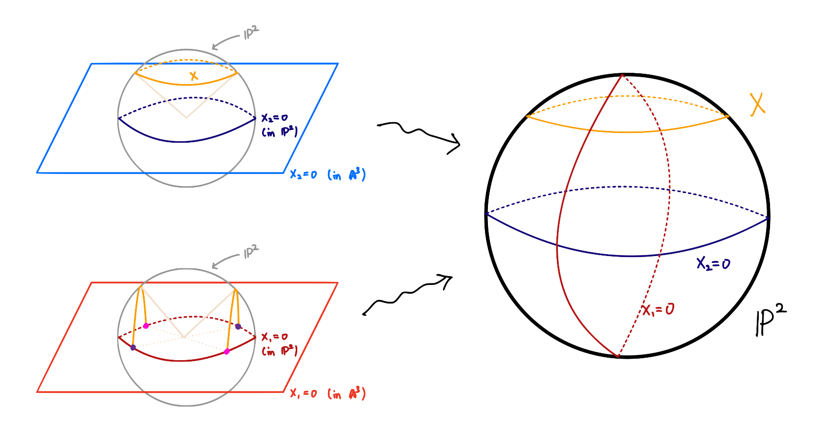
Example 11 To interpret the above proposition geometrically, let \(\mathbb{K}=\mathbb{R}\) and consider the conic \(X = Z(\x_0^2 + \x_1^2 - \x_2^2)\) in \(\mathbb{P}^2\).

This conic is the cone \(\x_0^2 + \x_1^2 = \x_2^2\) in \(\mathbb{A}^3\) expressed in homogeneous coordinates. Then Proposition 10 tells us how \(X\) looks in the standard open sets: to see what \(X\) looks like in \(U_i\), we simply substitute \(1\) for \(\x_i\) and regard the remaining \(n\) variables as coordinates on \(\mathbb{A}^n\). In particular we obtain the following.

1. In \(U_0\) and \(U_1\), the curve \(X\) is the hyperbola \(1+y^2-z^2=0\) and \(x^2+1-z^2=0\), respectively.
2. In \(U_2\), the curve \(X\) is the circle \(x^2+y^2=1\).

This happens because the equation \(\x_0^2 + \x_1^2 = \x_2^2\) in \(\mathbb{A}^3\) defines a cone, and intersecting it with the planes \(\x_0=1\), \(\x_1=1\), and \(\x_2=1\) yields hyperbolas and a circle, respectively.

On the other hand, we can also interpret this directly in \(\mathbb{P}^2\). To do so, we construct \(\mathbb{P}^2\) as follows. For points with \(\x_2\neq 0\), radially project onto the upper hemisphere satisfying \(\x_2>0\); for points with \(\x_2=0\), identify antipodal points. Through this construction, \(\mathbb{P}^2\) can be thought of as the plane \(\mathbb{A}^2\) corresponding to the surface of the upper hemisphere, together with the “line at infinity” \(\mathbb{P}^1\). Then the given cone first becomes a circle contained in the upper hemisphere via the first radial projection, and from this we know that \(X\) appears as a circle in \(\mathbb{P}^2\).

Of course, we could also have constructed \(\mathbb{P}^2\) by radially projecting points satisfying \(\x_0\neq 0\) onto the upper hemisphere with \(\x_0>0\), taking the points with \(\x_0=0\) as \(\mathbb{P}^1\). In this process, two semicircles would be drawn on the upper hemisphere, but the boundary points of these two semicircles would be identified as the same in the process of identifying the points with \(\x_0=0\), so in this picture too \(X\) would be a circle.

From this perspective, viewing \(X\) in \(U_i\) corresponds to removing the line at infinity \(\x_i=0\) from \(\mathbb{P}^2\). If we look at \(X\) in \(U_2\), then as we saw above, \(X\) does not meet the line at infinity \(\x_2=0\), so removing this line leaves a complete circle. However, if for example we remove the line at infinity \(\x_1=0\), then \(X\) meets \(\x_1\) at two points, and so removing these two points from the circle \(X\) and “unfolding” it yields a hyperbola.

Affine Cone

The preceding example shows how to view a curve in projective space within each affine open chart, but one may still find this somewhat less intuitive. Another way to understand a projective variety as a geometric object in affine space is to consider its affine cone.

Definition 12 The affine cone \(C(X) \subseteq \mathbb{A}^{n+1}\) of a projective variety \(X \subseteq \mathbb{P}^n\) is defined as follows:

\[C(X) = \{(x_0, \ldots, x_n) \in \mathbb{A}^{n+1} \setminus \{0\} \mid [x_0 : \cdots : x_n] \in X\} \cup \{0\}.\]

That is, \(C(X)\) is the union of all points in \(\mathbb{A}^{n+1}\) that appear when the points of \(X\) are expressed in homogeneous coordinates, together with the origin.

Example 13 The affine cone \(C(X)\) of the conic \(X = Z(\x_0^2 + \x_1^2 - \x_2^2) \subseteq \mathbb{P}^2\) from Example 11 is the cone \(\x_0^2 + \x_1^2 = \x_2^2\) in \(\mathbb{A}^3\).

The following then holds, and the proofs are not difficult.

Proposition 14 The affine cone \(C(X)\) of a projective variety \(X \subseteq \mathbb{P}^n\) satisfies the following properties:

1. (Homogeneity) \(C(X)\) consists of lines through the origin. That is, if \((x_0, \ldots, x_n) \in C(X)\) and \(\lambda \in \mathbb{K}\), then \((\lambda x_0, \ldots, \lambda x_n) \in C(X)\).

2. (Algebraic structure) If \(X = Z(F_1, \ldots, F_k)\), then \(C(X) = V(F_1, \ldots, F_k) \subseteq \mathbb{A}^{n+1}\), where the \(F_i\) are regarded as polynomials on \(\mathbb{A}^{n+1}\).

3. (Correspondence) The correspondence \(X \leftrightarrow C(X)\) gives a one-to-one correspondence between projective varieties and affine algebraic sets consisting of lines through the origin.

Through this proposition, we can indirectly study the properties of \(X\) by investigating the properties of its affine cone \(C(X)\).

Morphisms of Projective Varieties

Finally, we define morphisms of projective varieties. Earlier, when we defined projective algebraic sets, we saw that the zero set of a polynomial does not generally define a well-defined set on projective space; a similar issue arises when defining morphisms, and the solution is again homogeneous polynomials.

Definition 15 A function \(\varphi: X \to Y\) is a morphism between projective varieties \(X \subseteq \mathbb{P}^n\) and \(Y \subseteq \mathbb{P}^m\) if for each point \(x\) there exist suitable homogeneous polynomials \(F_0, \ldots, F_m\) of the same degree such that

\[\varphi(x) = [F_0(x) : \cdots : F_m(x)]\]

and for all \(x \in X\), the \(F_i(x)\) are not simultaneously zero.

If \(F_0, \ldots, F_m\) are all homogeneous polynomials of the same degree \(d\), then since \(F_i(\lambda x) = \lambda^d F_i(x)\), we have

\[[F_0(\lambda x) : \cdots : F_m(\lambda x)] = [\lambda^d F_0(x) : \cdots : \lambda^d F_m(x)] = [F_0(x) : \cdots : F_m(x)],\]

so well-definedness is guaranteed. The following examples are representative morphisms.

Example 16 First, the Veronese embedding (of degree 2) from \(\mathbb{P}^1\) to \(\mathbb{P}^2\),

\[[x:y]\mapsto [x^2: xy:y^2]\]

is a morphism between projective spaces. As another example, the Segre embedding from \(\mathbb{P}^1\times \mathbb{P}^1\) to \(\mathbb{P}^3\) is the morphism given by

\[([x:y], [u:v])\mapsto [xu: xv: yu: yv]\]

Example 17 Twisted cubic in \(\mathbb{P}^3\)

\[C = \{[1 : t : t^2 : t^3] \mid t \in \mathbb{K}\} \cup \{[0 : 0 : 0 : 1]\}\]

is the common zero locus of the three quadratic polynomials

\[\x_0 \x_2 - \x_1^2, \quad \x_0 \x_3 - \x_1 \x_2, \quad \x_1 \x_3 - \x_2^2\]

and is isomorphic to \(\mathbb{P}^1\). In fact, extending the notion of the Veronese embedding from Example 16 to \(d=3\),

\[[x:y]\mapsto [x^3: x^2y: xy^2: y^3]\]

is an isomorphism from \(\mathbb{P}^1\) to \(C\).

---

References

[Har] J. Harris, Algebraic Geometry: A First Course, Springer, 1992.
[Sha] I. R. Shafarevich, Basic Algebraic Geometry I: Varieties in Projective Space, Springer, 2013.
[Ful] W. Fulton, Algebraic Curves, 2008.